r - The Hong Kong Polytechnic University

displacement). The flow diagram of the software tools for longitudinal buffer responses monitoring is shown
in Figure 30 (lower part).
3.3.3 Software System for Data Interfacing and Analysis Execution
The software system for data interfacing and analysis execution, which is deployed in SHDMS-Server, is
customized for five functions: (i) retrieval of data and information from the rolling storage buffer (or the raw
data database as shown in Figure 45) in the SHDMS-Server to the DPCS-workstations in accordance with user’s
request, (ii) matching the retrieval data and information to each assigned customized software tools (i.e. the
software system for bridge structural system as described in Paragraph 3.3.2), (iii) execution of the requested
processing, analysis and plotting works, (iv) generation and/or storage of relevant monitoring reports. In the
application of this software system, the required input data and information by the user are: the tag-name of
sensors, the time durations for processing and analysis, the types of processing, analysis and plots required. This
approach not only minimizes the time for data retrieval, but also speeds up the works of data processing,
analysis and reporting works. The required types of data and tools for data interfacing and analysis execution are
shown in Figure 31.
3.4. Examples of Monitoring Results
In order to limit the scope of presentation, only eight examples of monitoring examples are presented. They are
selected because they have comparative large variations and therefore some of the major features of the
measurands and/or the bridge can be extracted. These eight examples are : (i) wind and weather monitoring –
basic steady wind and turbulence wind monitoring, (ii) highway traffic monitoring – highway loading spectrum,
(iii) static features monitoring – stress influence line determination, (iv) global dynamic features monitoring –
vertical flexural deck frequencies extraction, (v) stay force monitoring – stay cable forces distribution, (vi)
displacements monitoring – indirect approach of re-generating the global bridge deformed geometry, (vii)
fatigue damage monitoring, and (viii) permanent loads monitoring.
As all the customized software systems for SCB-WASHMS till now (May 2011) have not yet been completed
and handed over to Highways Department for operation and in order to avoid any contractual controversy, it is
declared that the following monitoring results are produced based on the measured data in Stonecutters Bridge
with the application of similar software tools used in the SHMS for Tsing Ma Bridge, Kap Shui Mun Bridge and
Ting Kau Bridge [Ref. 8, 34 and 35].
3.4.1 Wind and Weather Monitoring (Figures 32-33)
In this example, two outputs are presented. The first output, as shown in Figure 32, is the plot of wind rose
diagram basing on the monthly wind data in February 2011 obtained from the wind sensor: Ane(U3D) which is
located at the Southeast side of mid main span. The second output, as shown in Figure 32, is the plots of wind
power spectrum diagram and the integral length scale (based on the direct integration of the auto-covariance
function of the measured wind speeds) of the 2-hour wind data (21 October 2010 at 08:00-10:00 am) from the
wind sensor: Ane(U3D) which is located at Northeast of mid main span. This 2-hour wind data has a 10-minute
mean wind speed of 6.27 m/s with a turbulence intensity of 20.1%. The measured peak value of the spectrum is
at 0.0047 Hz; whereas the derived integral length scale is 75.2m, which is much less than the criteria for
buffeting response check.
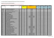
3.4.2 Highway Traffics Monitoring (Figures 34-35)
Figure 34 illustrates the highway traffic composition monitoring result in February 2011, and Figure 35
illustrates the corresponding estimated the fatigue damages in individual traffic lane. The sum of damage
(fatigue) ratios in six traffic lanes is 0.1714, which has been projected to 1-year’s damage ratio, and the
corresponding estimated fatigue life is 700 years (=120 years/0.1714, where 120-year is the design life of the
bridge), which is greater than the Engineer’s design fatigue life of 200~500 years at the fatigue assessment
point.
3.4.3 Global Static Features Monitoring (Figures 36-37)
The static features monitoring refers to the determination of the static influence displacement and stress
coefficients. Before, the opening of the Stonecutters Bridge to public traffic, load trials (including influence
lines measurements) had been carried [Ref. 37]. Figure 36 and 37 illustrate the tested and analyzed results of
-254-