texto: metodos numericos para ecuaciones diferenciales ordinarias

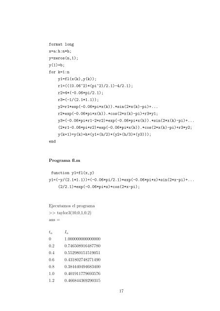
format long
x=a:h:n*h;
y=zeros(n,1);
y(1)=b;
for k=1:n
end
y1=fl(x(k),y(k));
r1=(((0.06^2)*(pi^2)/2.1)-4/2.1);
r2=4*(-0.06*pi/2.1);
r3=(-1/(2.1*1.1));
y2=r1*exp(-0.06*pi*x(k)).*sin(2*x(k)-pi)+...
r2*exp(-0.06*pi*x(k)).*cos(2*x(k)-pi)+r3*y1;
y3=(-0.06*pi*r1-2*r2)*exp(-0.06*pi*x(k)).*sin(2*x(k)-pi)+...
(2*r1-0.06*pi*r2)*exp(-0.06*pi*x(k)).*cos(2*x(k)-pi)+r3*y2;
y(k+1)=y(k)+h*(y1+(h/2)*(y2+(h/3)*(y3)));
Programa fl.m
function y1=fl(x,y)
y1=(-y/(2.1*1.1))+(-0.06*pi/2.1)*exp(-0.06*pi*x)*sin(2*x-pi)+...
(2/2.1)*exp(-0.06*pi*x)*cos(2*x-pi);
Ejecutamos el programa
>> taylor3(10,0,1,0.2)
ans =
tn
In
0 1.000000000000000
0.2 0.746508916487780
0.4 0.552980151519051
0.6 0.431802748271490
0.8 0.384440494683400
1.0 0.401911779693576
1.2 0.466844369290315
17