texto: metodos numericos para ecuaciones diferenciales ordinarias

posicion (m)
x 10−3
7
6
5
4
3
2
1
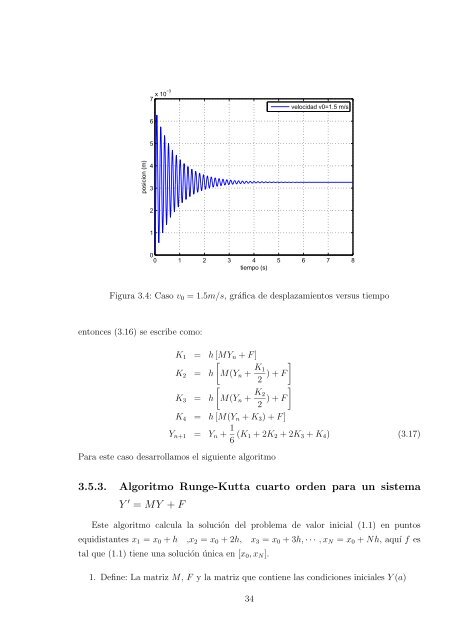
velocidad v0=1.5 m/s
0
0 1 2 3 4
tiempo (s)
5 6 7 8
Figura 3.4: Caso v0 = 1.5m/s, gráfica de desplazamientos versus tiempo
entonces (3.16) se escribe como:
K1 = h [MYn + F]
K2 = h M(Yn + K1
) + F
2
K3 = h M(Yn + K2
) + F
2
K4 = h [M(Yn + K3) + F]
Yn+1 = Yn + 1
6 (K1 + 2K2 + 2K3 + K4) (3.17)
Para este caso desarrollamos el siguiente algoritmo
3.5.3. Algoritmo Runge-Kutta cuarto orden para un sistema
Y ′ = MY + F
Este algoritmo calcula la solución del problema de valor inicial (1.1) en puntos
equidistantes x1 = x0 + h ,x2 = x0 + 2h, x3 = x0 + 3h, · · · ,xN = x0 + Nh, aquí f es
tal que (1.1) tiene una solución única en [x0,xN].
1. Define: La matriz M, F y la matriz que contiene las condiciones iniciales Y (a)
34