texto: metodos numericos para ecuaciones diferenciales ordinarias

More documents

Recommendations

Info

Program vibracion.m 1 2k m Base c 1 2k Figura 3.10: Modelo de un instrumento sísmico %Halla el movimiento y velocidad del instrumento sísmico clear; clc; format long k=40*10; w=5.81778; m=120;A=0.1;wn=sqrt(k/m);c=wn*m M=[0 1;-k/m -c/m]; Y(:,1)=[0;0]; h=0.1;n=1;t(1)=0;F=[0;A*(w^2)*sin(w*t(1))]; while t(n)
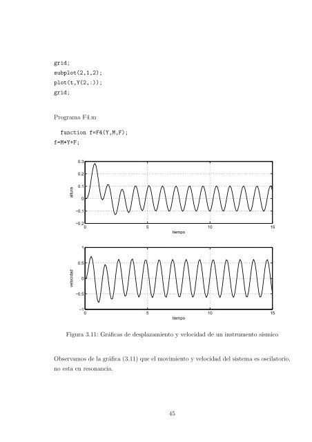
grid; subplot(2,1,2); plot(t,Y(2,:)); grid; Programa F4.m function f=F4(Y,M,F); f=M*Y+F; altura velocidad 0.3 0.2 0.1 0 −0.1 −0.2 0 5 10 15 tiempo 1 0.5 0 −0.5 −1 0 5 10 15 tiempo Figura 3.11: Gráficas de desplazamiento y velocidad de un instrumento sísmico Observamos de la gráfica (3.11) que el movimiento y velocidad del sistema es oscilatorio, no esta en resonancia. 45
Page 1 and 2: UNIVERSIDAD NACIONAL DEL CALLAO FAC
Page 3 and 4: 3.5.4. Monorriel de dos carros . .
Page 5 and 6: Resumen Las ecuaciones diferenciale
Page 7 and 8: Parte teórica o marco teórico 1 C
Page 9 and 10: 3. Parar xn+1 = xn + h yn+1 = yn +
Page 11 and 12: se reduce el error que se comete. 2
Page 13 and 14: 0.2 1.95962956e+000 0.3 2.93814836e
Page 15 and 16: Ejemplo Sea el problema de valor in
Page 17 and 18: 8. Una pieza metálica con una masa
Page 19 and 20: haciendo φ(x0) = y0 φ(x1) ≈ y1
Page 21 and 22: 2. Aproximar y(0) de y ′ = cosx
Page 23 and 24: format long x=a:h:n*h; y=zeros(n,1)
Page 25 and 26: ) Use las respuestas obtenidas en e
Page 27 and 28: Capítulo 3 Métodos de Runge-Kutta
Page 29 and 30: 3.2. Método Modificado de Euler yn
Page 31 and 32: Ejemplo 1. Sea la ecuación diferen
Page 33 and 34: se resuelve utilizando el método d
Page 35 and 36: e. Para j = 1, 2,...,m hacer f. Par
Page 37 and 38: end T=[t]; y=[w]; w(j)=c(j) for i=1
Page 39 and 40: donde posicion (m) x 10−3 6 5 4 3
Page 41 and 42: 2. Para n=0,...,N-1, hacer 3. Parar
Page 43 and 44: Figura 3.8: Diagrama de cuerpo libr
Page 45 and 46: B2=10000;B3=10000;B1=5000; B23=500;
Page 47 and 48: 19 1.9 9.5572e-002 8.5217e-002 8.02
Page 49: 3.5.6. Instrumento sísmico En la f
Page 53 and 54: ) Resuelva por el método de Runge-
Page 55 and 56: esuelva el PVI con el método de Ru
Page 57 and 58: las aproximaciones wi+1 y ¯wi+1 a
Page 59 and 60: si se repiten los pasos, q se elige
Page 61 and 62: los parámetros en forma adecuada.
Page 63 and 64: La entrada al algoritmo es la toler
Page 65 and 66: Materiales y Métodos La informaci
Page 67 and 68: a mantenerse constante a partir del
Page 69 and 70: iteraciones con h = 0.1. En conclus
Page 71 and 72: [KEN 92] KEN NAGLE,R..Fundamentos d
Page 73 and 74: x=-pi:0.1:pi; >> y=x.*cos(x); >> pl
Page 75 and 76: Apéndice B:Unicidad de la solució

texto: metodos numericos para ecuaciones diferenciales ordinarias

You also want an ePaper? Increase the reach of your titles

Delete template?

Save as template?