Modélisation, analyse mathématique et simulations numériques de ...

tel-00656013, version 1 - 3 Jan 2012
4.2 Numerical schemes and main results 99
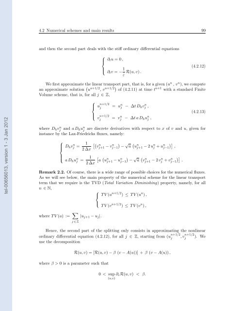
and then the second part deals with the stiff ordinary differential equations
⎧
⎪⎨
⎪⎩
∂tu = 0,
∂tv = − 1
ε R(u,v).
(4.2.12)
We first approximate the linear transport part, that is, for a given(u n , v n ), we compute
an approximate solution u n+1/2 , v n+1/2 of (4.2.11) at time t n+1 with a standard Finite
Volume scheme, that is, for all j ∈ Z,
where Dhv n j and aDhu n j
⎧
⎪⎨
⎪⎩
u n+1/2
j
v n+1/2
j
= u n j − ∆tDhv n j ,
= v n j − ∆taDhu n j ,
(4.2.13)
are discrete derivatives with respect to x of v and u, given for
instance by the Lax-Friedrichs fluxes, namely:
⎧
⎪⎨
⎪⎩
Dhv n j = 1
2∆x
aDhu n j
= 1
2∆x
n
vj+1 −v n √ n
j−1 − a uj+1 −2u n j +u n
j−1 ,
n
a uj+1 −u n √
n
j−1 − a vj+1 −2v n j +vn
j−1 .
Remark 2.2. Of course, there is a wide range of possible choices for the numerical fluxes.
As we will see below, the main property of the numerical scheme for the linear transport
term that we require is the TVD (Total Variation Diminishing) property, namely, for all
n ∈ N,
⎧
⎨ TV(u n+1/2 ) ≤ TV(u n ),
where TV(u) :=
j∈Z
⎩
|uj+1 −uj|.
TV(v n+1/2 ) ≤ TV(v n ),
Hence, the second part of the splitting only consists in approximating the nonlinear
ordinary differential equation (4.2.12), for all j ∈ Z, starting from (u n+1/2
j ,v n+1/2
j ). We
use the decomposition
where β > 0 is a parameter such that
R(u,v) = [R(u,v)−β (v −A(u))] + β (v −A(u)),
0 < sup ∂vR(u,v) < β.
(u,v)