Modélisation, analyse mathématique et simulations numériques de ...

tel-00656013, version 1 - 3 Jan 2012
5.3 Time Fourier analysis and boundary layer approximations 153
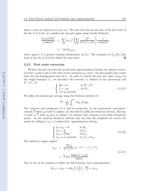
where c does not depend on k nor on l. We now treat the second part of the first term of
the rhs of (5.3.14): in a similar way one gets again using Cauchy-Schwartz
|ˆvp,l(1)| 2 |b| 2
≤ |am,l|
|sinh(b)| 2 2
|b| 2
4π4m4 +|b| 4
1
|sinh(b)| 2
m
≤ cφl 2
L 2 (0,1) ,
where again c is a generic constant independent on k,l. The estimates of |ˆv ′ p,l (0)| (last
term of the rhs of (5.3.14)) follow the same lines.
5.3.3 First order correction
We have already seen that the zeroth order approximation contains two distinct sources
of errors: a part is due to the order of the extension û0,k in Ωε \Ω0 and another part comes
from the non homogeneous rest on Γε. In order to correct the non zero value of û0,k on
the rough boundary Γε, we introduce the corrector β, defined on the microscopic cell
Z + ∪Γ∪P ⎧
⎨ ∆β = 0 in Z
⎩
+ ∪P ,
β = −y2 on P0,
(5.3.15)
β is y1-periodic.
We define the microscopic average along the fictitious interface Γ:
β = 1
2π
2π
0
m
β(y1,0)dy1.
The existence and uniqueness of β, and its properties, as the exponential convergence
towards β when y2 tends to infinity, are described in [40] and references therein. Because
β tends to β when y2 goes to infinity, we subtract this constant in the final asymptotic
ansatz. As the constant should be relevant only far from the roughness we correct the
ansatz by adding to û1,k a “counter-flow” approximation solving:
⎧
⎪⎨
⎪⎩
The solution is again explicit:
Lk û1,k = 0 in Ω0,
û1,k = 0 on Γ1,
û1,k = βMk on Γ0,
û1,k is x1-periodic on Γin ∪Γout.
û1,k = −βMk
e r −e −r
= βMk
e −r e rx2 −e r e −rx2
sinh(r(1+x2))
sinh(r)
Now we are in the position to define the full boundary layer approximation :
Ûǫ,k := û0,k +εMk
β
x
ε
−β
.
+εû1,k.
(5.3.16)
(5.3.17)