Modélisation, analyse mathématique et simulations numériques de ...

tel-00656013, version 1 - 3 Jan 2012
4.3 A priori estimates 101
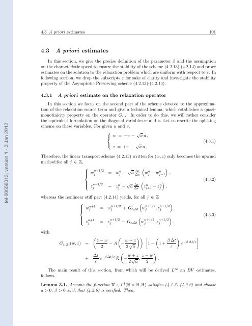
4.3 A priori estimates
In this section, we give the precise definition of the parameter β and the assumption
on the characteristic speed to ensure the stability of the scheme (4.2.13)-(4.2.14) and prove
estimates on the solution to the relaxation problem which are uniform with respect to ε. In
following section, we drop the subscripts ε for sake of clarity and investigate the stability
property of the Asymptotic Preserving scheme (4.2.13)-(4.2.14).
4.3.1 A priori estimate on the relaxation operator
In this section we focus on the second part of the scheme devoted to the approximation
of the relaxation source term and give a technical lemma, which establishes a quasimonotinicity
property on the operator Gε,s. In order to do this, we will rather consider
the equivalent formulation on the diagonal variables w and z. Let us rewrite the splitting
scheme on these variables. For given u and v,
⎧
⎨ w = −v −
⎩
√ au,
z = +v − √ (4.3.1)
au.
Therefore, the linear transport scheme (4.2.13) written for (w,z) only becomes the upwind
method:for all j ∈ Z,
⎧
⎪⎨ w
⎪⎩
n+1/2
j = wn j −√a ∆t
∆x wn j −wn
j−1 ,
zn j+1 −zn
j ,
(4.3.2)
z n+1/2
j
= z n j +√ a ∆t
∆x
whereas the nonlinear stiff part (4.2.14) yields, for all j ∈ Z
with
⎧
⎪⎨
⎪⎩
Gε,∆t(w,z) =
w n+1
j = w n+1/2
j
z n+1
j
= z n+1/2
j
+ Gε,∆t
− Gε,∆t
w n+1/2
j ,z n+1/2
j
w n+1/2
j ,z n+1/2
j ,
z −w
2 −A
− w+z
2 √
1− 1+
a
β∆t
ε
+ ∆t
ε e−β∆t/ε R
− w+z
2 √ z −w
,
a 2
.
,
e −β∆t/ε
(4.3.3)
The main result of this section, from which will be derived L ∞ an BV estimates,
follows.
Lemma 3.1. Assume the function R ∈ C 1 (R×R,R) satisfies (4.1.3)-(4.2.2) and choose
a > 0, β > 0 such that (4.2.6) is verified. Then,