Modélisation, analyse mathématique et simulations numériques de ...

tel-00656013, version 1 - 3 Jan 2012
110 An Asymptotic Preserving scheme
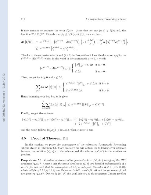
It now remains to evaluate the error En j (ε). Using that for any (u,v) ∈ I(N0,a0), the
function R ∈ C1 (R + ,R) such that β0 ≤ ∂vR(u,v) ≤ β, then we have
∆t n
Ej (ε)
−β∆t/ε
= e
−
v n+1/2
j −A(u n+1/2
j )
1+ β∆t
ε
≤ e −β0∆t/ε
v n+1/2
j −A(u n+1/2
j ) .
+ ∆t
ε R
u n+1/2
j ,v n+1/2
j
,
Thanks to the estimates (4.4.1) and (4.4.2) in Proposition 4.1 on the deviation applied to
v n+1/2 −A(u n+1/2 ) which is also valid in the asymptotic ε → 0, it yields
v n+1/2 −A(u n+1/2 ⎧
⎨ 0
δ
)L1 ≤
⎩
L1 + C∆t if n = 0,
C∆t if n > 0.
Then, we get for k ≥ 0 and ε ≤ ∆t,
∆x∆t E k j (ε)
≤
j∈Z
⎧
⎨
⎩
Hence summing over 0 ≤ k ≤ n, it gives
n
∆x∆t
k=0 j∈Z
Finally, we get the estimate
E k ε,∆t
e −β0∆t/ε δ 0 L 1 + C∆t
if k = 0,
Ce −β0∆t/ε ∆t if k > 0.
≤ e −β0∆t/ε 0
δ
L1 + Ct n+1 .
w ε h (tn )−wh(t n ) L 1 +z ε h (tn )−zh(t n ) L 1 ≤ w ε h (0)−wh(0) L 1 +z ε h (0)−zh(0) L 1
+ 2e −β0∆t/ε δ 0 L 1 + Ct n
and the result follows (u ε h ,vε h ) → (uh,vh), when ε goes to zero.
4.5 Proof of Theorem 2.4
In this section, we prove the convergence of the relaxation Asymptotic Preserving
scheme stated in Theorem 2.4. More precisely, we will obtain the following error estimate
between the solution (u ε h ,vε h ) to the scheme and the solution (uε ,v ε ) to the continuous
problem.
Proposition 5.1. Consider a discretization parameter h = (∆t,∆x) satisfying the CFL
are bounded independently of ε
condition (4.2.8). Assume that the initial conditions uε 0 ,vε 0
in BV(R) and such that the assumption (4.2.5) is satisfied. Consider R ∈ C1 (R×R,R),
which satisfies (4.1.3)-(4.2.2) and the characteristic speed √ a > 0 and the parameter β > 0
are given by (4.2.6). Denote by (uε ,vε ) the weak solution to the relaxation Cauchy problem