Modélisation, analyse mathématique et simulations numériques de ...

tel-00656013, version 1 - 3 Jan 2012
4.4 Trend to equilibrium 107
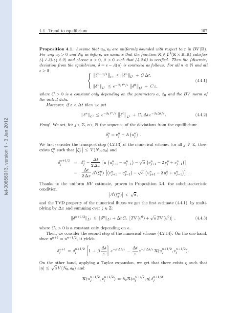
Proposition 4.1. Assume that u0,v0 are uniformly bounded with respect to ε in BV(R).
For any a0 > 0 and N0 as before, we assume that the function R ∈ C 1 (R×R,R) satisfies
(4.1.3)-(4.2.2) and choose a > 0, β > 0 such that (4.2.6) is verified. Then the (discrete)
deviation from the equilibrium, δ = v−A(u) is controled as follows. For all n ∈ N and all
ε > 0 ⎧ ⎨
⎩
δ n+1/2 L 1 ≤ δ n L 1 + C∆t,
δ n L 1 ≤ e −β0t n /ε δ 0 L 1 + Cε.
(4.4.1)
where C > 0 is a constant only depending on the parameters a, β0 and the BV norm of
the initial data.
Moreover, if ε < ∆t then we get
δ n L 1 ≤ e −β0t n /ε δ 0 L 1 + Ca∆te −β0∆t/ε . (4.4.2)
Proof. We set, for j ∈ Z, n ∈ N the sequence of the deviations from the equilibrium:
δ n j = vn j −Au n j .
We first consider the transport step (4.2.13) of the numerical scheme: for all j ∈ Z, there
exists ξn j such that
n
ξ
j ≤ V(N0,a0) and
δ n+1/2
j
= δ n j − ∆t
2∆x
n
a uj+1 −u n √ n
j−1 − a vj+1 −2v n j +v n
j−1
− ∆t
2∆x A′ (ξ n j ) v n j+1 −vn j−1
√
n
− a uj+1 −2u n j +un
j−1 .
Thanks to the uniform BV estimate, proven in Proposition 3.4, the subcharacteristic
condition
A ′ (ξ n j ) < √ a,
and the TVD property of the numerical fluxes we get the first estimate (4.4.1), by multiplying
by ∆x and summing over j ∈ Z:
δ n+1/2 L 1 ≤ δ n L 1 +∆tCa
TV(v 0 )+ √ aTV(u 0 ) , (4.4.3)
where Ca > 0 is a constant only depending on a.
Then, we consider the second step of the numerical scheme (4.2.14). On the one hand,
since u n+1 = u n+1/2 , it yields
δ n+1
j = δ n+1/2
j
1 + β ∆t
ε
e −β∆t/ε − ∆t
ε e−β∆t/ε R(u n+1/2
j ,v n+1/2
j ).
On the other hand, applying a Taylor expansion, we get that there exists η such that
|η| ≤ √ aV(N0,a0) and:
R(u n+1/2
j ,v n+1/2
j ) = ∂vR(u n+1/2
j ,η)δ n+1/2
j .