- Page 2 and 3:
Springer Handbook of Acoustics
- Page 4 and 5:
Springer Handbook of Acoustics Thom
- Page 6 and 7:
Foreword The present handbook cover
- Page 8 and 9:
List of Authors Iskander Akhatov No
- Page 10 and 11:
Philippe Roux Université Joseph Fo
- Page 12 and 13:
XIV Contents 3.7 Attenuation of Sou
- Page 14 and 15:
XVI Contents 10 Concert Hall Acoust
- Page 16 and 17:
XVIII Contents 17.8 Physical Modeli
- Page 18 and 19:
XX Contents 24.5 Free-Field Microph
- Page 20 and 21:
XXII List of Abbreviations K KDP po
- Page 22 and 23:
Introduction 1. Introduction to Aco
- Page 24 and 25:
of noise have been the subject of c
- Page 26 and 27:
in order to understand how objectiv
- Page 28 and 29:
A Brief 2. A Brief History of Acous
- Page 30 and 31:
of 350 m/s for the speed of sound [
- Page 32 and 33:
number and relative strength of its
- Page 34 and 35:
To his contemporaries, Koenig was p
- Page 36 and 37:
Probably the most important use of
- Page 38 and 39:
piezoelectric ceramic compositions
- Page 40 and 41:
surveys together [2.46]. Masking of
- Page 42 and 43:
ther of computer music, since he de
- Page 44 and 45:
Basic 3. Linear Basic Linear Acoust
- Page 46 and 47:
M average molecular weight n unit v
- Page 48 and 49:
a) b) S v.n ∆t ∆S V |v| ∆t n
- Page 50 and 51:
temperature, q =−κ∇T , (3.16)
- Page 52 and 53:
The equivalent density M/V is conse
- Page 54 and 55:
Basic Linear Acoustics 3.3 Equation
- Page 56 and 57:
Because any vector field may be dec
- Page 58 and 59:
The latter and (3.84), in a manner
- Page 60 and 61:
assumed to have no ambient motion,
- Page 62 and 63:
Because the friction associated wit
- Page 64 and 65:
3.5 Waves of Constant Frequency One
- Page 66 and 67:
3.5.4 Time Averages of Products Whe
- Page 68 and 69:
as well as symmetry considerations,
- Page 70 and 71:
The auxiliary internal variables th
- Page 72 and 73:
Then the transient at a distant pos
- Page 74 and 75:
ω ′ = 0, and this is consistent
- Page 76 and 77:
1.0 10 -1 10 -2 10 -3 10 -4 10 -5 A
- Page 78 and 79:
This yields the interpretation that
- Page 80 and 81:
direction of propagation when a pla
- Page 82 and 83:
so the time-averaged incident energ
- Page 84 and 85:
Although the simple result of (3.31
- Page 86 and 87:
ut, also in keeping with the linear
- Page 88 and 89:
equation, the two differential equa
- Page 90 and 91:
Rodrigues relation, one has �1
- Page 92 and 93:
for the derivative.) In the asympto
- Page 94 and 95:
The differential scattering cross s
- Page 96 and 97:
elow) is F(t) = (2c) 1/2 �t −
- Page 98 and 99:
0.5 0 -0.5 -1.0 -1.5 0 Y0(η) (π/2
- Page 100 and 101:
is the Wronskian for the Bessel and
- Page 102 and 103:
The function qS is termed the sourc
- Page 104 and 105:
The appropriate identification for
- Page 106 and 107:
where jℓ is the spherical Bessel
- Page 108 and 109:
this subtlety taken into account, o
- Page 110 and 111:
U(x) Basic Linear Acoustics 3.15 Wa
- Page 112 and 113:
is ordinarily valid. With these ass
- Page 114 and 115:
along rays. These can be regarded a
- Page 116 and 117:
A(x0) x0 A(x) Fig. 3.53 Sketch of a
- Page 118 and 119:
possible, and one where neither the
- Page 120 and 121:
which is independent of the z-coord
- Page 122 and 123:
[3.108], and Carslaw [3.109]. In th
- Page 124 and 125:
where C(X)andS(X) are the Fresnel i
- Page 126 and 127:
Fig. 3.60 Characteristic diffractio
- Page 128 and 129:
of elastic solids, Trans. Camb. Phi
- Page 130 and 131:
3.101 J.B. Keller: Geometrical acou
- Page 132 and 133:
114 Part A Propagation of Sound Par
- Page 134 and 135:
116 Part A Propagation of Sound Par
- Page 136 and 137:
118 Part A Propagation of Sound Par
- Page 138 and 139:
120 Part A Propagation of Sound Par
- Page 140 and 141:
122 Part A Propagation of Sound Par
- Page 142 and 143:
124 Part A Propagation of Sound Par
- Page 144 and 145:
126 Part A Propagation of Sound Par
- Page 146 and 147:
128 Part A Propagation of Sound Par
- Page 148 and 149:
130 Part A Propagation of Sound Par
- Page 150 and 151:
132 Part A Propagation of Sound Par
- Page 152 and 153:
134 Part A Propagation of Sound Par
- Page 154 and 155:
136 Part A Propagation of Sound Par
- Page 156 and 157:
138 Part A Propagation of Sound Par
- Page 158 and 159:
140 Part A Propagation of Sound Par
- Page 160 and 161:
142 Part A Propagation of Sound Par
- Page 162 and 163:
144 Part A Propagation of Sound Par
- Page 164 and 165:
146 Part A Propagation of Sound Par
- Page 166 and 167:
Underwater 5. Underwater Acoustics
- Page 168 and 169:
5.1 Ocean Acoustic Environment The
- Page 170 and 171:
Long-Range Propagation Paths Figure
- Page 172 and 173:
tal direction, there is no loss ass
- Page 174 and 175:
equivalent circuit, as shown in Fig
- Page 176 and 177:
Attenuation á (dB/km) 1000 100 10
- Page 178 and 179:
5.2.5 Ambient Noise There are essen
- Page 180 and 181:
ubble natural acoustic resonance ω
- Page 182 and 183:
a bubbly medium (and for the simple
- Page 184 and 185:
As discussed, because detection inv
- Page 186 and 187:
(1/A)∇ 2 A ≪ K 2 )sothat(5.34)
- Page 188 and 189:
water, where the deep sound channel
- Page 190 and 191:
egion in the form p(r, z) = ψ(r, z
- Page 192 and 193:
5.4.6 Propagation and Transmission
- Page 194 and 195:
tegration interval. The source puls
- Page 196 and 197:
5.6 SONAR Array Processing Signal p
- Page 198 and 199:
former output is: �∞ b(θ,t) =
- Page 200 and 201:
Fig. 5.37 Angle-versus-time represe
- Page 202 and 203:
5.7 Active SONAR Processing Depth M
- Page 204 and 205:
a factor when there is a reverberan
- Page 206 and 207:
depth measurements that correspond
- Page 208 and 209:
along the cross-shelf track taken b
- Page 210 and 211:
time as a result of multiple paths,
- Page 212 and 213:
technique is very sensitive, and ex
- Page 214 and 215:
Fig. 5.57a,b Typical echogram obtai
- Page 216 and 217:
Frequency (Hz) 150 100 50 0 0 a) b)
- Page 218 and 219:
out. These data allow for study of
- Page 220 and 221:
5.59 G. Raleigh, J.M. Cioffi: Spati
- Page 222 and 223:
Physical 6. Physical Acou Acoustics
- Page 224 and 225:
where I is the intensity of the sou
- Page 226 and 227:
Wave velocity The wall exerts a dow
- Page 228 and 229:
destructively interfered with one a
- Page 230 and 231:
or: � � p2 � rms SPL = 10 log
- Page 232 and 233:
6.1.4 Wave Propagation in Solids Si
- Page 234 and 235:
where c is again the wave speed and
- Page 236 and 237:
measured. Some resonances are cause
- Page 238 and 239:
as 50 µmto5µm through one oscilla
- Page 240 and 241:
the number of false positives and m
- Page 242 and 243:
with the small mass), and frequency
- Page 244 and 245:
Laser Lens 1 Circular aperture Fig.
- Page 246 and 247:
Ground ring Insulator Sample Resist
- Page 248 and 249:
Energy ratio 1.0 0.8 0.6 0.4 Calcul
- Page 250 and 251:
terms. In this equation γ is the r
- Page 252 and 253:
directly. The nonlinearity paramete
- Page 254 and 255:
Thermoacoust 7. Thermoacoustics The
- Page 256 and 257:
Table 7.1 The acoustic-electric ana
- Page 258 and 259:
walls of the pores. (Positive G ind
- Page 260 and 261:
a) b) c) C reso d) δtherm e) p 0 U
- Page 262 and 263:
a) b) UA,l c) d) E 0 Q A Q A TA TA
- Page 264 and 265:
tor. This eliminates the need to le
- Page 266 and 267:
to this consumption of acoustic pow
- Page 268 and 269:
The traditional Stirling refrigerat
- Page 270 and 271:
Washington 1986) pp. 550-554, Softw
- Page 272 and 273:
258 Part B Physical and Nonlinear A
- Page 274 and 275:
260 Part B Physical and Nonlinear A
- Page 276 and 277:
262 Part B Physical and Nonlinear A
- Page 278 and 279:
264 Part B Physical and Nonlinear A
- Page 280 and 281:
266 Part B Physical and Nonlinear A
- Page 282 and 283:
268 Part B Physical and Nonlinear A
- Page 284 and 285:
270 Part B Physical and Nonlinear A
- Page 286 and 287:
272 Part B Physical and Nonlinear A
- Page 288 and 289:
274 Part B Physical and Nonlinear A
- Page 290 and 291:
276 Part B Physical and Nonlinear A
- Page 292 and 293:
278 Part B Physical and Nonlinear A
- Page 294 and 295:
280 Part B Physical and Nonlinear A
- Page 296 and 297:
282 Part B Physical and Nonlinear A
- Page 298 and 299:
284 Part B Physical and Nonlinear A
- Page 300 and 301:
286 Part B Physical and Nonlinear A
- Page 302 and 303:
288 Part B Physical and Nonlinear A
- Page 304 and 305:
290 Part B Physical and Nonlinear A
- Page 306 and 307:
292 Part B Physical and Nonlinear A
- Page 308 and 309:
294 Part B Physical and Nonlinear A
- Page 310 and 311:
296 Part B Physical and Nonlinear A
- Page 312 and 313:
Acoustics 9. Acoustics in Halls for
- Page 314 and 315:
parameters, so we can assist in bui
- Page 316 and 317:
weeks or even years is less reliabl
- Page 318 and 319:
9.3.1 Reverberation Time Reverberan
- Page 320 and 321:
selected). A distance different fro
- Page 322 and 323:
ing sound, as will naturally be exp
- Page 324 and 325:
of the sound fields. Consequently,
- Page 326 and 327:
e derived from interrupted noise de
- Page 328 and 329:
Acoustics in Halls for Speech and M
- Page 330 and 331:
espectively, can be calculated from
- Page 332 and 333:
ated by the architects. However, on
- Page 334 and 335:
of C and G. However, as all the ind
- Page 336 and 337:
F b d F n I S Fb Fn S d F n/F b d/d
- Page 338 and 339:
HS S èn ã d0 P0 rn Position of ey
- Page 340 and 341:
Time T (s) 2.5 2 1.5 1 5 10 15 Acou
- Page 342 and 343:
floor can be tilted to reduce volum
- Page 344 and 345:
ÄLcurv (dB) 10 8 6 4 2 0 -2 -4 -6
- Page 346 and 347:
Acoustics in Halls for Speech and M
- Page 348 and 349:
Acoustics in Halls for Speech and M
- Page 350 and 351:
Acoustics in Halls for Speech and M
- Page 352 and 353:
Seating capacity 2662 1 915 + 324 2
- Page 354 and 355:
Acoustics in Halls for Speech and M
- Page 356 and 357:
4 3 2 1 Acoustics in Halls for Spee
- Page 358 and 359:
cially in auditoria with T values l
- Page 360 and 361:
esonance (AR)andmultichannel reverb
- Page 362 and 363:
Concert 10. Concert Hall Acoustics
- Page 364 and 365:
Concert Hall Acoustics Based on Sub
- Page 366 and 367:
0 0 Concert Hall Acoustics Based on
- Page 368 and 369:
mately by Concert Hall Acoustics Ba
- Page 370 and 371:
Concert Hall Acoustics Based on Sub
- Page 372 and 373:
10.1.5 Specialization of Cerebral H
- Page 374 and 375:
The other (n − 1) bits indicated
- Page 376 and 377:
As for the conflicting requirements
- Page 378 and 379:
have mainly been concerned with tem
- Page 380 and 381:
a) c) S S -4.3 -2.8 -2.0 -3.5 -3dB
- Page 382 and 383:
Concert Hall Acoustics Based on Sub
- Page 384 and 385:
Concert Hall Acoustics Based on Sub
- Page 386 and 387:
Concert Hall Acoustics Based on Sub
- Page 388 and 389:
Concert Hall Acoustics Based on Sub
- Page 390 and 391:
Concert Hall Acoustics Based on Sub
- Page 392 and 393:
Concert Hall Acoustics Based on Sub
- Page 394 and 395:
Concert Hall Acoustics Based on Sub
- Page 396 and 397:
a model of the auditory-brain syste
- Page 398 and 399:
Building 11. Building Acou Acoustic
- Page 400 and 401:
Pressure Maximum Minimum 0 D Distan
- Page 402 and 403:
Table 11.1 Absorption coefficients
- Page 404 and 405:
Absorption coefficient α 1 0 Frequ
- Page 406 and 407:
is of key importance in rooms where
- Page 408 and 409:
Table 11.4 Transmission loss and ST
- Page 410 and 411:
TL of wall - (TL of door, window or
- Page 412 and 413:
Table 11.7 Generalized noise reduct
- Page 414 and 415:
Masking sound pressure level (dB) 5
- Page 416 and 417:
As for the room criterion (RC) meth
- Page 418 and 419:
11.5 Noise Control Methods for Buil
- Page 420 and 421:
Neoprene pads (30 durometer) with a
- Page 422 and 423:
Concrete Caulk around perimeter Vib
- Page 424 and 425:
Trim board to conceal gap (fasten o
- Page 426 and 427:
Gypsum board partition (as schedule
- Page 428 and 429:
Double-layer ribbed or waffle neopr
- Page 430 and 431:
11.6 Acoustical Privacy in Building
- Page 432 and 433:
Table 11.9 AI,SIIandPIforopenplanof
- Page 434 and 435:
Electronic sound masking in plenum
- Page 436 and 437:
E 1179 Standard Specification for S
- Page 438 and 439:
430 Part D Hearing and Signal Proce
- Page 440 and 441:
432 Part D Hearing and Signal Proce
- Page 442 and 443:
434 Part D Hearing and Signal Proce
- Page 444 and 445:
436 Part D Hearing and Signal Proce
- Page 446 and 447:
438 Part D Hearing and Signal Proce
- Page 448 and 449:
440 Part D Hearing and Signal Proce
- Page 450 and 451:
442 Part D Hearing and Signal Proce
- Page 452 and 453:
444 Part D Hearing and Signal Proce
- Page 454 and 455:
446 Part D Hearing and Signal Proce
- Page 456 and 457:
448 Part D Hearing and Signal Proce
- Page 458 and 459:
450 Part D Hearing and Signal Proce
- Page 460 and 461:
452 Part D Hearing and Signal Proce
- Page 462 and 463:
454 Part D Hearing and Signal Proce
- Page 464 and 465:
456 Part D Hearing and Signal Proce
- Page 466 and 467:
Psychoacoust 13. Psychoacoustics Ps
- Page 468 and 469:
Absolute threshold (dB SPL) 100 90
- Page 470 and 471:
the signal. By using this off-cente
- Page 472 and 473:
is as a crude indicator of the exci
- Page 474 and 475:
Relative response (dB) 100 90 80 70
- Page 476 and 477:
In a variation of this procedure, t
- Page 478 and 479:
Level of matching noise (dB) 100 90
- Page 480 and 481:
13.4 Temporal Processing in the Aud
- Page 482 and 483:
Most models include an initial stag
- Page 484 and 485:
The components were either uniforml
- Page 486 and 487:
(Frequency DL)/ERBN 0.2 0.1 0.05 0.
- Page 488 and 489:
elaborate place models have been pr
- Page 490 and 491:
13.6 Timbre Perception 13.6.1 Time-
- Page 492 and 493:
the duplex theory of sound localiza
- Page 494 and 495:
harmonic (by shifting the frequency
- Page 496 and 497:
sive. While some studies have been
- Page 498 and 499:
sentences (see Fig. 13.20). They va
- Page 500 and 501:
components is usually only perceive
- Page 502 and 503:
References 13.1 ISO 389-7: Acoustic
- Page 504 and 505:
13.74 D. Ronken: Monaural detection
- Page 506 and 507:
asymmetric function, J. Acoust. Soc
- Page 508 and 509:
13.211 J. Vliegen, A.J. Oxenham: Se
- Page 510 and 511:
504 Part D Hearing and Signal Proce
- Page 512 and 513:
506 Part D Hearing and Signal Proce
- Page 514 and 515:
508 Part D Hearing and Signal Proce
- Page 516 and 517:
510 Part D Hearing and Signal Proce
- Page 518 and 519:
512 Part D Hearing and Signal Proce
- Page 520 and 521:
514 Part D Hearing and Signal Proce
- Page 522 and 523:
516 Part D Hearing and Signal Proce
- Page 524 and 525:
518 Part D Hearing and Signal Proce
- Page 526 and 527:
520 Part D Hearing and Signal Proce
- Page 528 and 529:
522 Part D Hearing and Signal Proce
- Page 530 and 531:
524 Part D Hearing and Signal Proce
- Page 532 and 533:
526 Part D Hearing and Signal Proce
- Page 534 and 535:
528 Part D Hearing and Signal Proce
- Page 536 and 537:
530 Part D Hearing and Signal Proce
- Page 538 and 539:
534 Part E Music, Speech, Electroac
- Page 540 and 541:
536 Part E Music, Speech, Electroac
- Page 542 and 543:
538 Part E Music, Speech, Electroac
- Page 544 and 545:
540 Part E Music, Speech, Electroac
- Page 546 and 547:
542 Part E Music, Speech, Electroac
- Page 548 and 549:
544 Part E Music, Speech, Electroac
- Page 550 and 551:
546 Part E Music, Speech, Electroac
- Page 552 and 553:
548 Part E Music, Speech, Electroac
- Page 554 and 555:
550 Part E Music, Speech, Electroac
- Page 556 and 557:
552 Part E Music, Speech, Electroac
- Page 558 and 559:
554 Part E Music, Speech, Electroac
- Page 560 and 561:
556 Part E Music, Speech, Electroac
- Page 562 and 563:
558 Part E Music, Speech, Electroac
- Page 564 and 565:
560 Part E Music, Speech, Electroac
- Page 566 and 567:
562 Part E Music, Speech, Electroac
- Page 568 and 569:
564 Part E Music, Speech, Electroac
- Page 570 and 571:
566 Part E Music, Speech, Electroac
- Page 572 and 573:
568 Part E Music, Speech, Electroac
- Page 574 and 575:
570 Part E Music, Speech, Electroac
- Page 576 and 577:
572 Part E Music, Speech, Electroac
- Page 578 and 579:
574 Part E Music, Speech, Electroac
- Page 580 and 581:
576 Part E Music, Speech, Electroac
- Page 582 and 583:
578 Part E Music, Speech, Electroac
- Page 584 and 585:
580 Part E Music, Speech, Electroac
- Page 586 and 587:
582 Part E Music, Speech, Electroac
- Page 588 and 589:
584 Part E Music, Speech, Electroac
- Page 590 and 591:
586 Part E Music, Speech, Electroac
- Page 592 and 593:
588 Part E Music, Speech, Electroac
- Page 594 and 595:
590 Part E Music, Speech, Electroac
- Page 596 and 597:
592 Part E Music, Speech, Electroac
- Page 598 and 599:
594 Part E Music, Speech, Electroac
- Page 600 and 601:
596 Part E Music, Speech, Electroac
- Page 602 and 603:
598 Part E Music, Speech, Electroac
- Page 604 and 605:
600 Part E Music, Speech, Electroac
- Page 606 and 607:
602 Part E Music, Speech, Electroac
- Page 608 and 609:
604 Part E Music, Speech, Electroac
- Page 610 and 611:
606 Part E Music, Speech, Electroac
- Page 612 and 613:
608 Part E Music, Speech, Electroac
- Page 614 and 615:
610 Part E Music, Speech, Electroac
- Page 616 and 617:
612 Part E Music, Speech, Electroac
- Page 618 and 619:
614 Part E Music, Speech, Electroac
- Page 620 and 621:
616 Part E Music, Speech, Electroac
- Page 622 and 623:
618 Part E Music, Speech, Electroac
- Page 624 and 625:
620 Part E Music, Speech, Electroac
- Page 626 and 627:
622 Part E Music, Speech, Electroac
- Page 628 and 629:
624 Part E Music, Speech, Electroac
- Page 630 and 631:
626 Part E Music, Speech, Electroac
- Page 632 and 633:
628 Part E Music, Speech, Electroac
- Page 634 and 635:
630 Part E Music, Speech, Electroac
- Page 636 and 637:
632 Part E Music, Speech, Electroac
- Page 638 and 639:
634 Part E Music, Speech, Electroac
- Page 640 and 641:
636 Part E Music, Speech, Electroac
- Page 642 and 643:
638 Part E Music, Speech, Electroac
- Page 644 and 645:
640 Part E Music, Speech, Electroac
- Page 646 and 647:
642 Part E Music, Speech, Electroac
- Page 648 and 649:
644 Part E Music, Speech, Electroac
- Page 650 and 651:
646 Part E Music, Speech, Electroac
- Page 652 and 653:
648 Part E Music, Speech, Electroac
- Page 654 and 655:
650 Part E Music, Speech, Electroac
- Page 656 and 657:
652 Part E Music, Speech, Electroac
- Page 658 and 659:
654 Part E Music, Speech, Electroac
- Page 660 and 661:
656 Part E Music, Speech, Electroac
- Page 662 and 663:
658 Part E Music, Speech, Electroac
- Page 664 and 665:
660 Part E Music, Speech, Electroac
- Page 666 and 667:
662 Part E Music, Speech, Electroac
- Page 668 and 669:
664 Part E Music, Speech, Electroac
- Page 670 and 671:
666 Part E Music, Speech, Electroac
- Page 672 and 673:
The 16. The Human Human Voice in Sp
- Page 674 and 675:
uation, the effect of gravity is in
- Page 676 and 677:
piratory muscles (the internal inte
- Page 678 and 679:
Mean Ps (cm H2O) 50 40 30 20 10 0 D
- Page 680 and 681:
Glottal flow Closed Opening Open Cl
- Page 682 and 683:
Transglottal airflow (l/s) 0.4 0.2
- Page 684 and 685:
Mean spectrum level (dB) -30 -40 -5
- Page 686 and 687:
20 10 0 -10 -20 -30 -40 -50 0 i y u
- Page 688 and 689:
Mean level (dB) 0 -10 -20 -30 -40 1
- Page 690 and 691:
This topic was addressed by Ladefog
- Page 692 and 693:
Fig. 16.29 Acoustic consequences of
- Page 694 and 695:
Bass i e u Alto Tenor o ε œ æ Th
- Page 696 and 697:
100 80 60 40 20 0 -20 100 80 60 40
- Page 698 and 699:
tours for [� ]and[Ù ] sampled at
- Page 700 and 701:
Rapp [16.100] asked three native sp
- Page 702 and 703:
Utterance command T0 T3 Accent comm
- Page 704 and 705:
The # symbol indicates the possibil
- Page 706 and 707:
Second formant frequency (Hz) 2500
- Page 708 and 709:
tional rather than absolute (à la
- Page 710 and 711:
16.7 P. Ladefoged, M.H. Draper, D.
- Page 712 and 713:
esonance imaging: Vowels, J. Acoust
- Page 714 and 715:
16.139 A. Eriksson: Aspects of Swed
- Page 716 and 717:
Computer 17. Computer Mu Music This
- Page 718 and 719:
Quantum step Amplitude Quantization
- Page 720 and 721:
Some might notice that linear inter
- Page 722 and 723:
pers, textbooks, patents, etc. Furt
- Page 724 and 725:
0:00.0 0.5 0 Computer Music 17.3 Ad
- Page 726 and 727:
(0,0) (0,1) (1,1) (0,2) (1,2) (0,3)
- Page 728 and 729:
synthesizing vocoder. The main diff
- Page 730 and 731:
x(n) + z -1 z -1 Scattering junctio
- Page 732 and 733:
230 Hz FOF 1100 Hz FOF 1700 Hz FOF
- Page 734 and 735:
0 y + - Computer Music 17.8 Physica
- Page 736 and 737:
-1 (1-ß )×length Velocity + Veloc
- Page 738 and 739:
0 -30 (dB) -60 0 1.5 3 4.5 (kHz) Fi
- Page 740 and 741:
17.10 Composition The history of co
- Page 742 and 743:
and variance of the features can be
- Page 744 and 745:
17.20 J.L. Kelly Jr., C.C. Lochbaum
- Page 746 and 747:
Audio 18. Audio and Electroacoustic
- Page 748 and 749:
Alexander Graham Bell filed his pat
- Page 750 and 751:
on magnetic stripes. A common arran
- Page 752 and 753:
60 40 20 0 SPL-sound pressure level
- Page 754 and 755:
Interaural intensity difference (dB
- Page 756 and 757:
with equalization, without incurrin
- Page 758 and 759:
Fig. 18.8 Sine wave with crossover
- Page 760 and 761:
18.3.8 Dynamic Range Dynamic range
- Page 762 and 763:
Directly actuated type Diaphragm ty
- Page 764 and 765:
effective pickup pattern of the arr
- Page 766 and 767:
attempts to apply complementary com
- Page 768 and 769:
Most of the issues relating to spea
- Page 770 and 771:
nificant design considerations. At
- Page 772 and 773:
Some appreciation of the performanc
- Page 774 and 775:
pre-digital reverberators were elec
- Page 776 and 777:
and ‘s’ in English text - may b
- Page 778 and 779:
content of rest of the signal spect
- Page 780 and 781:
cross the head, in opposite directi
- Page 782 and 783:
18.2 J. Sterne: The Audible Past (D
- Page 784 and 785:
18.71 T. Sporer: Creating, assessin
- Page 786 and 787:
786 Part F Biological and Medical A
- Page 788 and 789:
788 Part F Biological and Medical A
- Page 790 and 791:
790 Part F Biological and Medical A
- Page 792 and 793:
792 Part F Biological and Medical A
- Page 794 and 795:
794 Part F Biological and Medical A
- Page 796 and 797:
796 Part F Biological and Medical A
- Page 798 and 799:
798 Part F Biological and Medical A
- Page 800 and 801:
800 Part F Biological and Medical A
- Page 802 and 803:
802 Part F Biological and Medical A
- Page 804 and 805:
804 Part F Biological and Medical A
- Page 806 and 807:
806 Part F Biological and Medical A
- Page 808 and 809:
808 Part F Biological and Medical A
- Page 810 and 811:
810 Part F Biological and Medical A
- Page 812 and 813:
812 Part F Biological and Medical A
- Page 814 and 815:
814 Part F Biological and Medical A
- Page 816 and 817:
816 Part F Biological and Medical A
- Page 818 and 819:
818 Part F Biological and Medical A
- Page 820 and 821:
820 Part F Biological and Medical A
- Page 822 and 823:
822 Part F Biological and Medical A
- Page 824 and 825:
824 Part F Biological and Medical A
- Page 826 and 827:
826 Part F Biological and Medical A
- Page 828 and 829:
828 Part F Biological and Medical A
- Page 830 and 831:
830 Part F Biological and Medical A
- Page 832 and 833:
832 Part F Biological and Medical A
- Page 834 and 835:
834 Part F Biological and Medical A
- Page 836 and 837:
836 Part F Biological and Medical A
- Page 838 and 839:
Medical 21. Medical Acous Acoustics
- Page 840 and 841:
21.1 Introduction to Medical Acoust
- Page 842 and 843:
Auscultation location Right & left
- Page 844 and 845:
portance. The Strouhal number has b
- Page 846 and 847:
Fig. 21.3 Phono-cardiograph transdu
- Page 848 and 849:
Amplitude 8 6 4 2 0 -2 -4 -6 Displa
- Page 850 and 851:
λ1 = c1 / fus θ1 λ2 = c2 / fus
- Page 852 and 853:
lood flow can be resolved if the si
- Page 854 and 855:
vided in the image thickness direct
- Page 856 and 857:
not as predicted, because the wave
- Page 858 and 859:
Fig. 21.18a,b Quadrature Doppler de
- Page 860 and 861:
a) b) c) 100 0 V mV 10 0 a = 13 a =
- Page 862 and 863:
Ultrasound contact gel Position enc
- Page 864 and 865:
a) 10 cm b) c) 10 cm Fig. 21.32a-c
- Page 866 and 867:
a) Pin B Pin A Ultrasound line b) M
- Page 868 and 869:
Organ Patient Ultrasound transducer
- Page 870 and 871:
systems cannot tell the difference
- Page 872 and 873:
40 µm can be resolved. For a 10 kH
- Page 874 and 875:
a) b) c) d) Medical Acoustics 21.4
- Page 876 and 877:
Fig. 21.54 Doppler spectral wavefor
- Page 878 and 879:
10 20 30 10 20 30 Pre-exercise B-mo
- Page 880 and 881:
Vibrations in a punctured artery De
- Page 882 and 883:
the veins and diffuse into the inte
- Page 884 and 885:
21.5.3 Agitated Saline and Patent F
- Page 886 and 887:
transported by those cells and/or r
- Page 888 and 889:
1 0.8 0.6 0.4 0.2 0 Relative power
- Page 890 and 891:
High intensity focused ultrasound h
- Page 892 and 893:
a) b) c) Fig. 21.74a-c B-mode imagi
- Page 894 and 895:
provided simple metrics for the lik
- Page 896 and 897:
thickness of the carotid arteries,
- Page 898 and 899:
Structural 22. Structural Acoustics
- Page 900 and 901:
Structural Acoustics and Vibrations
- Page 902 and 903:
Magnitude (arb. units) 1.4 1.2 1.0
- Page 904 and 905:
This does not include the case wher
- Page 906 and 907:
the mass matrix is taken to be cons
- Page 908 and 909:
Magnitude (dB) -10 -30 -50 0 1 2 3
- Page 910 and 911:
where D(ω) = ω 4 − 2iω 3�
- Page 912 and 913:
form y(x, t) = � Φn(x)qn(t) . (2
- Page 914 and 915:
first to solve the wave equation (2
- Page 916 and 917:
5 3 1 -1 -3 -5 0 1 2 3 4 5 6 7 8 9
- Page 918 and 919:
conditions at each end) are necessa
- Page 920 and 921:
from which we can derive through (2
- Page 922 and 923:
In this case, the eigenfrequencies
- Page 924 and 925:
of radiation modes and their link w
- Page 926 and 927:
Finally, the displacement is ˜ξ(x
- Page 928 and 929:
notes the value of this eigenmode a
- Page 930 and 931:
Pm = ˙Q H [Rs + Ra] ˙Q , (22.262)
- Page 932 and 933:
where and Ra = 2ζaω0 M Z(s) = zL
- Page 934 and 935:
Radiated Power. The mean acoustic p
- Page 936 and 937:
(22.318) can be written ξ(x, y, t)
- Page 938 and 939:
Denoting the eigenfrequencies and e
- Page 940 and 941:
Magnitude (arb. units) 3 2 1 0 -1 -
- Page 942 and 943:
for any real symmetric tensor Xij.
- Page 944 and 945:
F(N) 1 0.5 0 -0.5 -1 -1 -0.8 -0.6 -
- Page 946 and 947:
whose solution is θ1 = A cos ωτ.
- Page 948 and 949:
4.5 3.5 2.5 1.5 A 0.5 0 0.5 1.0 1.5
- Page 950 and 951:
Equations (22.423) are usually writ
- Page 952 and 953:
3. As the amplitude reaches the top
- Page 954 and 955:
Shallow Spherical Shells and Plates
- Page 956 and 957:
22.20 L. Cremer, M. Heckl: Structur
- Page 958 and 959:
Noise Noise is discussed in terms o
- Page 960 and 961:
where the overbars represent time a
- Page 962 and 963:
Typical outdoor setting A-weighted
- Page 964 and 965:
90 dB(A)” is widely used, and imp
- Page 966 and 967:
Microphone, amplifier and A/D conve
- Page 968 and 969:
When each segment of the measuremen
- Page 970 and 971:
found from � LW = Lp + 10 log A +
- Page 972 and 973:
surement method is the ultimate use
- Page 974 and 975: An intensity analyzer is more compl
- Page 976 and 977: 23.2.5 Criteria for Noise Emissions
- Page 978 and 979: Table 23.5 Table of limit values fr
- Page 980 and 981: a) Air flows freely to rotor Weak t
- Page 982 and 983: Static efficiency normalized to its
- Page 984 and 985: ful applications. Good results are
- Page 986 and 987: Table 23.8 Crossover speeds for var
- Page 988 and 989: Reduction of airplane engine noise
- Page 990 and 991: A variety of materials are used to
- Page 992 and 993: ∆LF (dB) 0 -10 -20 α -30 0.05 0.
- Page 994 and 995: Absorption coefficient 1.0 0.8 0.6
- Page 996 and 997: high enough that there is little so
- Page 998 and 999: 23.4.4 Criteria for Noise Immission
- Page 1000 and 1001: Table 23.10 (cont.) Some features o
- Page 1002 and 1003: Noise 23.4 Noise and the Receiver 1
- Page 1004 and 1005: view of administrative procedures r
- Page 1006 and 1007: provides recommendations for a foll
- Page 1008 and 1009: sound power levels of noise sources
- Page 1010 and 1011: 23.68 ISO: ISO 9296:1988 Acoustics
- Page 1012 and 1013: in impedance tubes - Part 2: Transf
- Page 1014 and 1015: 23.194 Commission of the European C
- Page 1016 and 1017: 1022 Part H Engineering Acoustics P
- Page 1018 and 1019: 1024 Part H Engineering Acoustics P
- Page 1020 and 1021: 1026 Part H Engineering Acoustics P
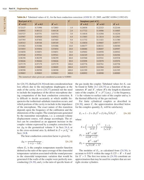
- Page 1022 and 1023: 1028 Part H Engineering Acoustics P
- Page 1026 and 1027: 1032 Part H Engineering Acoustics P
- Page 1028 and 1029: 1034 Part H Engineering Acoustics P
- Page 1030 and 1031: 1036 Part H Engineering Acoustics P
- Page 1032 and 1033: 1038 Part H Engineering Acoustics P
- Page 1034 and 1035: 1040 Part H Engineering Acoustics P
- Page 1036 and 1037: 1042 Part H Engineering Acoustics P
- Page 1038 and 1039: 1044 Part H Engineering Acoustics P
- Page 1040 and 1041: 1046 Part H Engineering Acoustics P
- Page 1042 and 1043: 1048 Part H Engineering Acoustics P
- Page 1044 and 1045: 1050 Part H Engineering Acoustics P
- Page 1046 and 1047: Sound 25. Intens Sound Intensity So
- Page 1048 and 1049: Under such conditions the intensity
- Page 1050 and 1051: a) Pressure and particle velocity 0
- Page 1052 and 1053: τ is a dummy time variable. The ca
- Page 1054 and 1055: Error in intensity (dB) 5 0 -5 -10
- Page 1056 and 1057: 8 7 6 5 4 3 2 1 0 -1 -2 -3 Error du
- Page 1058 and 1059: crophones are calibrated with a pis
- Page 1060 and 1061: Sound power level (dB re 1 pW) 72 7
- Page 1062 and 1063: it is relatively straightforward si
- Page 1064 and 1065: intensity normal to the source. Thi
- Page 1066 and 1067: 25.9 W. Maysenhölder: The reactive
- Page 1068 and 1069: 25.77 ISO: ISO 11205 Acoustics - No
- Page 1070 and 1071: 1078 Part H Engineering Acoustics P
- Page 1072 and 1073: 1080 Part H Engineering Acoustics P
- Page 1074 and 1075:
1082 Part H Engineering Acoustics P
- Page 1076 and 1077:
1084 Part H Engineering Acoustics P
- Page 1078 and 1079:
1086 Part H Engineering Acoustics P
- Page 1080 and 1081:
1088 Part H Engineering Acoustics P
- Page 1082 and 1083:
1090 Part H Engineering Acoustics P
- Page 1084 and 1085:
1092 Part H Engineering Acoustics P
- Page 1086 and 1087:
1094 Part H Engineering Acoustics P
- Page 1088 and 1089:
1096 Part H Engineering Acoustics P
- Page 1090 and 1091:
1098 Part H Engineering Acoustics P
- Page 1092 and 1093:
Optical 27. Optical Methods Metho f
- Page 1094 and 1095:
course also present in ordinary hol
- Page 1096 and 1097:
Optical Methods for Acoustics and V
- Page 1098 and 1099:
Optical Methods for Acoustics and V
- Page 1100 and 1101:
Optical Methods for Acoustics and V
- Page 1102 and 1103:
50 100 150 200 250 300 350 400 450
- Page 1104 and 1105:
a) b) Optical Methods for Acoustics
- Page 1106 and 1107:
nm 1000 0 -1000 150 y (mm) 100 50 O
- Page 1108 and 1109:
Optical Methods for Acoustics and V
- Page 1110 and 1111:
Optical Methods for Acoustics and V
- Page 1112 and 1113:
Laser Optical Methods for Acoustics
- Page 1114 and 1115:
References 27.1 E.F.F. Chladni: Die
- Page 1116 and 1117:
27.75 E.-L.Johansson, L. Benckert,
- Page 1118 and 1119:
1128 Part H Engineering Acoustics P
- Page 1120 and 1121:
1130 Part H Engineering Acoustics P
- Page 1122 and 1123:
1132 Part H Engineering Acoustics P
- Page 1124 and 1125:
1134 Part H Engineering Acoustics P
- Page 1126 and 1127:
1136 Part H Engineering Acoustics P
- Page 1128 and 1129:
1138 Part H Engineering Acoustics P
- Page 1130 and 1131:
About the Authors Iskander Akhatov
- Page 1132 and 1133:
Neville H. Fletcher Chapter F.19 Au
- Page 1134 and 1135:
Brian C. J. Moore Chapter D.13 Univ
- Page 1136 and 1137:
Detailed Contents List of Abbreviat
- Page 1138 and 1139:
3.8.3 Acoustic Power ..............
- Page 1140 and 1141:
4.8.3 Typical Speed of Sound Profil
- Page 1142 and 1143:
7.3 Engines .......................
- Page 1144 and 1145:
10 Concert Hall Acoustics Based on
- Page 1146 and 1147:
13.4 Temporal Processing in the Aud
- Page 1148 and 1149:
15.2.5 String-Bridge-Body Coupling
- Page 1150 and 1151:
19.6 Birds ........................
- Page 1152 and 1153:
22.4.5 Combinations of Elementary S
- Page 1154 and 1155:
24.8 Overall View on Microphone Cal
- Page 1156 and 1157:
Subject Index 3 dB bandwidth 463 A
- Page 1158 and 1159:
British Medical Ultrasound Society
- Page 1160 and 1161:
electric circuit analogues - acoust
- Page 1162 and 1163:
hyperspeech 703 hypospeech 703 I IA
- Page 1164 and 1165:
- participation factors 909 - stiff
- Page 1166 and 1167:
- musical instruments 541 - musical
- Page 1168 and 1169:
- nonlinear vibrations 957 - plate
- Page 1170 and 1171:
subjective preference theory 353 su