10. Appendix

Solution to Problem 9.2
Solution to Problem 9.2 665
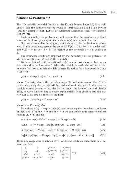
This 1D periodic potential (known as the Kronig-Penney Potential) is so wellknown
that the solutions can be found in textbooks on Solid State Physics
(see, for example, Ref. [7.14]) or Quantum Mechanics (see, for example,
Ref. [9.19]).
First, to simplify the problem we will assume that the solutions are Bloch
waves of the form: Ê exp(ikx)u(x) where u(x) is a periodic function.
Next we assume that the origin x 0 is chosen to be the beginning of one
well. In this coordinate system the potential V(x) 0 for 0 x a (the well)
and V(x) V for a x b. The period of the potential a b is defined as
d.
The boundary conditions imposed by the periodicity of the potential on
u(x) are: u(0) u(d) and u ′ (0) u′ (d).
We have defined u(0) u(‰) and u(d) u(d ‰) where, in both cases,
‰ is 0 and in the limit ‰ ⇒ 0. When the particle is inside the well we expect
its wave function to satisfy the Schrödinger Equation for a free particle (since
V(x) 0):
Ê(x) A exp(ik1x) B exp(ik1x) (9.2a)
where E (k1) 2 /2m is the particle energy. We will now assume that E V
so that classically the particle will be confined inside the well. In this case the
particle cannot penetrate into the barrier under the laws of classical physics.
Thus, its wave function has to decay exponentially with distance into the barrier.
Let us assume solutions of the form:
Ê(x) C exp(Îx) D exp(Îx) (9.2b)
where V E (Î) 2 /2m.
By writing u(x) exp(ikx)Ê(x) and imposing the boundary conditions
on u(x) and u ′ (x) atx 0 and at x a we can obtain four linear equations
relating A, B, C and D:
A B exp(ikd))[C exp(Îd) D exp(Îd)] (9.2c)
ik1(A B) Î exp(ikd)[C exp(Îd) D exp(Îd)] (9.2d)
A exp(ik1a) B exp(ik1a) C exp(Îa) D exp(Îa) (9.2e)
ik1[A exp(ik1a) B exp(ik1a)] Î[C exp(Îa) D exp(Îa)] (9.2f)
These 4 homogenous equations have non-trivial solutions when their determinant
vanishes:
1
1 ed(Îik) ed(Îik) k1 k1 Î
i
ed(Îik)
Î
i ed(Îik)
eik1a eik1a eÎa eÎa
0
(9.2g)
k1e ik1a k1e ik1a Î
i eÎa
Î
i eÎa