- Page 1:
CHAPTER 1 INTRODUCTION BY LOUIS N.
- Page 4 and 5:
4 IN TRODUC7”ION [SEC.1.2 flik~c
- Page 6 and 7:
6 INTRODUCTION [SEC.1.3 pulse leaki
- Page 8 and 9:
8 INTRODUCTION [SEC.1.4 antenna is
- Page 10 and 11:
10 INTRODUCTION [SEC.14 step in out
- Page 12 and 13:
12 INTRODUCTION [SEC.1.5 where high
- Page 14 and 15:
14 INTRODUCTION [SEC.1.6 England, F
- Page 16 and 17:
16 INTRODUCTION [SEC.1°7 Microwave
- Page 18 and 19:
CHAPTER 2 THE lU.DAR EQUATION BY E.
- Page 20 and 21:
20 THE RADAR EQUATION [SEC.22 radia
- Page 22 and 23:
22 THE RADAR EQUATION [SEC.25 Again
- Page 24 and 25:
24 THE RADAR EQUATION [SEC.2.5 time
- Page 26 and 27:
26 THE RADAR EQUATION [SEC.2.5 smal
- Page 28 and 29:
28 THE RADAR EQUATION [SEC.!2.7 lim
- Page 30 and 31:
30 THE RADAR EQUATION [SEC.28 Anoth
- Page 32 and 33:
32 THE RADAR EQUATION [SEC.28 first
- Page 34 and 35:
34 TIIE RADAR EQUATION [Sm. 29 the
- Page 36 and 37:
36 THE RADAR EQUATION [SEC.2.10 (Vo
- Page 38 and 39:
38 THE RADAR EQUATION [SEC.210 prac
- Page 40 and 41:
40 THE RADAR EQUATION [SEC.2.10 tai
- Page 42 and 43:
42 THE RADAR EQUATION [SEC.2.11 swe
- Page 44 and 45:
44 THE RADAR EQUATION [SEC.2.11 res
- Page 46 and 47:
46 THE RADAR EQUATION [SEC.211 Alth
- Page 48 and 49:
48 THE RADAR EQUATION [SEC.212 othe
- Page 50 and 51:
50 THE RADAR EQUATION [SEC.212 The
- Page 52 and 53:
52 THE RADAR EQUATION [SEC. 2.12 Th
- Page 54 and 55:
54 THE RADAR EQUATION [SEC.213 smal
- Page 56 and 57:
56 THE RADAR EQUATION [SEC. 2.14 an
- Page 58 and 59:
58 THE RADAR EQUATION [SEC.2.15 not
- Page 60 and 61:
60 TIIE RADAR EQUATION [SEC.2.15 wt
- Page 62 and 63:
62 THE RADAR EQUATION [SEC.215 per
- Page 64 and 65:
64 PROPERTIES OF RADAR TARGETS [SEC
- Page 66 and 67:
66 PROPERTIES OF RADAR TARGET,S [SE
- Page 68 and 69:
68 PROPERTIES OF RADAR TARGETS [SEC
- Page 70 and 71:
PROPERTIES OF RADAR TARGETS [SEC.37
- Page 72 and 73:
72 PROPERTIES OF RADAR TARGETS [SEC
- Page 74 and 75:
74 PROPERTIES OF RADAR TARGETS [SEC
- Page 76 and 77:
76 PROPERTIES OF RADAR TARGETS [SEC
- Page 78 and 79:
78 PROPERTIES OF RADAR TARGETS [SEC
- Page 80 and 81:
80 PROPERTIES OF RADAR TARGETS [SEC
- Page 82 and 83:
82 PROPERTIES OF RADAR TARGETS [SEC
- Page 84 and 85:
84 PROPERTIES OF RADAR TARGETS [SEC
- Page 86 and 87:
86 PROPERTIES OF RADAR TARGETS [SEC
- Page 88 and 89:
88 PROPERTIES OF R.41~.l R T.-lRGE~
- Page 90 and 91:
90 PROPERTIES OF RADAR TARGETS [SEC
- Page 92 and 93:
92 PROPERTIES OF RA1l.4R TARGETS [S
- Page 94 and 95:
94 PROPERTIES OF RADAR TARGETS [SEC
- Page 96:
96 PROPERTIES OF RADAR TARGETS [SEC
- Page 99 and 100:
SEC.315] STRUCTURES 99 example, the
- Page 101 and 102:
SF,C. 3.16] CITIES 101 reflection w
- Page 103 and 104:
SEC. 3.16] CITIES 103 signal repres
- Page 105:
SEC. 3.16] CITIES 105 four signals
- Page 108 and 109:
108 PROPERTIES OF RADAR TARGETS [SE
- Page 112:
112 PROPERTIES OF RADAR TARGETS [SE
- Page 116 and 117:
CHAPTER 4 LIMITATIONS OF PULSE RADA
- Page 118 and 119:
118 LIMITATIONS OF PULSE RADAR [SEC
- Page 120 and 121:
120 LIMITATIONS OF PULSE RADAR [SEC
- Page 122 and 123:
122 LIMITATIONS OF PC’LSE RADAR [
- Page 124 and 125:
124 LIMITATIONS OF PULSE RADAR [SEC
- Page 126 and 127:
126 LIMITATIONS OF PULSE RADAR [SEC
- Page 128 and 129:
128 C-W RADAR SYSTEMS [SEC. 5.1 tar
- Page 130 and 131:
130 C-W RADAR SYSTEMS [sm. 53 point
- Page 132 and 133:
132 C-W RADAR S’YSTEMS [SEC.56 bi
- Page 134 and 135:
134 C-W RADAR SYSTEMS [SEC. 56 tran
- Page 136 and 137:
136 C-W RADAR SYSTEMS [SEC. 5.6 int
- Page 138 and 139:
138 C-W RADAR SYSTEMS [SEC, 5.6 rel
- Page 140 and 141:
140 C-W RADAR SYSTEMS [SEC 37 and j
- Page 142 and 143:
142 C-II’ RADAR SYSTEMS [SEC. 57
- Page 144 and 145:
144 C-W RADAR SYSTE.JfS [SEC. 58 gi
- Page 146 and 147:
146 C-W RADAR SYSTEMS [SEC. 58 Modu
- Page 148 and 149:
148 C-T RA DAR S YSTE.lf S [SEC. 59
- Page 150 and 151:
150 C-W RADAR SYSTEMS [SEC. 5.11 cy
- Page 152 and 153:
152 C-W RADAR SYSTEMS [SEC.5.11 Now
- Page 154 and 155:
154 C-W RADAR SYSTEMS [SEC.5.11 exc
- Page 156 and 157:
156 C-W RADAR SYSTEMS [SEC. 5.11 in
- Page 158 and 159:
158 C-W RADAR SYSTEMS [SEC. 5.12 Pu
- Page 160 and 161:
CHAPTER 6 THE GATHERING AND PRESENT
- Page 162 and 163:
162 THE GATHERING AND PRESENTATION
- Page 164 and 165:
164 THE GATHERING AND PRESENTATION
- Page 166 and 167:
166 THE GATHERING AND PRESENTATION
- Page 168 and 169:
168 THE GATHERING AND pRESENTA TION
- Page 170 and 171:
~70 THE GATHERING AND PRESENTA TION
- Page 173 and 174:
SEC. 66] PLANE DISPLAYS INVOLVING E
- Page 175 and 176:
SEC. 69] IiARLY AIRCRAFT-WARNING RA
- Page 177 and 178:
SEC. 69] EARLY AIRCRAFT-WARNING RAD
- Page 179 and 180:
f$Ec. 69] EARLY AIRCRAFT-WARNING RA
- Page 181 and 182:
SEC. 6.9] EARLY AIRCRAFT-WARNING RA
- Page 183 and 184:
SEC. 6.10] PPI RADAR FOR SEARCH, CO
- Page 185 and 186:
SEC. 6.11] HEIGHT-FINDING INVOLVING
- Page 187 and 188:
SEC.6.12] HEIGHT-FINDING WITH A FRE
- Page 189 and 190:
SEC.6.12] HEIGHT-FINDING WITH A FRE
- Page 191 and 192:
SEC.6.12] HEIGHT-FINDING WITH A FRE
- Page 193 and 194:
- - -— . .. —-— - .. —-.
- Page 195 and 196:
SEC. 612] HEIGHT-FINDING J~ITH A FR
- Page 197 and 198:
SEC. 6.13] HOMING 197 ber of the pa
- Page 199 and 200:
SEC.6.13] HOMING 199 usually made t
- Page 201 and 202:
SEC. 6.13] HOMING 201 application,
- Page 203 and 204:
SEC. 6.14] PRECISION TRACKING OF A
- Page 205 and 206:
SEC.6.14] PRECISION TRACKING OF A S
- Page 207 and 208:
SEC. 614] PRECISION TRACKING OF A S
- Page 209 and 210:
f$Ec. 614] PRECISION TRACKING OF A
- Page 211 and 212:
SEC. 615] PRECISION TRACKING DURING
- Page 213 and 214:
CHAPTER 7 THE EMPLOYMENT OF RADAR D
- Page 215 and 216:
SEC.72] AIDS TO INDIVIDUAL NAVIGATI
- Page 217 and 218:
SEC. 7.2] AIDS TO INDIVIDUAL NAVIGA
- Page 219 and 220:
SEC. 73] AIDS TO PLOTTING AND CONTR
- Page 221 and 222:
SEC.7.3] AIDS TO PLOTTING AND CONTR
- Page 223 and 224:
SEC.7.3] AIDS TO PLOTTING AND CONTR
- Page 225 and 226:
SEC. 7.4] THE RELAY OF RADAR DISPLA
- Page 227 and 228:
SEC. 7.51 RA DAR IN THE RAF FIGHTER
- Page 229 and 230:
SEC. 7.6] THE U.S. TACTICAL AIR COM
- Page 231 and 232:
SEC. 7.6] THE U.S. TACTICAL AIR COM
- Page 233 and 234:
SEC. 7.6] THE U.S. TACTICAL AIR COM
- Page 235:
SEC.7.6] THE U.S. TACTICAL AIR COMM
- Page 238 and 239:
238 THE EMPLOYMENT OF RA DAR DATA [
- Page 240 and 241:
240 THE EMPLOYiWENT OF RADAR DATA [
- Page 242 and 243:
242 THE EMPLOYMENT OF RADAR DATA [S
- Page 244 and 245:
244 RADAR BEACONS [SEC. 8 duration
- Page 246 and 247:
246 RADAR BEACONS [SEC. 8.1 beacons
- Page 248 and 249:
248 RADAR BEACONS [SEC.8.1 4. Porta
- Page 250 and 251:
250 RADAR BEACONS [SEC.8.2 Table 8.
- Page 252 and 253:
252 RADAR BEACONS [SEC.84 restricte
- Page 254 and 255:
254 RADAR BEACONS [SEC. 85 radar se
- Page 256 and 257:
256 RADAR BEACONS [SEC.85 In the ca
- Page 258:
258 It Al)AIt BEACONS [S,,c, S3 Sim
- Page 261 and 262:
SEC. 86] FREQUENCY CONSIDERATIONS 2
- Page 263 and 264:
SEC. 87] INTERR~A TION CODES 263 wi
- Page 265 and 266:
SEC. 8.9] TRAFFIC CAPACITY 265 diff
- Page 267 and 268:
SEC.8.9] TRAFFIC CAPACITY 267 which
- Page 270 and 271:
270 RADAR BEACONS [SEC. 810 range a
- Page 272 and 273:
272 ANTENNAS, SCANNERS, A.VD STABIL
- Page 274 and 275:
274 ANTENNAS, SCANNERS, AND ST ABIL
- Page 276 and 277:
276 ANTENNAS, SCANNERS, AND STABILI
- Page 278 and 279:
278 ANTENNAS, SCANNERS, AND STABILI
- Page 280 and 281:
280 ANTENNAS, SCANNERS, AND STABILI
- Page 282 and 283:
282 ANTENNAS, SCANNERS, AND STABILI
- Page 284 and 285:
284 ANTENNAS, SCANNERS, AND STABILI
- Page 286 and 287:
286 ANTENNAS, SCANNERS, AND STABILI
- Page 288:
288 ANTENNAS, SCANNERS, AND STABILI
- Page 291 and 292:
SEC. 913] THE AN/APQ-7 (EAGLE) SCAN
- Page 293 and 294:
SEC.913] THE AN/APQ-7 (EAGLE) SCANN
- Page 295 and 296:
SEC. 9.14] SCHWA RZSCHILD ANTENNA 2
- Page 297 and 298:
SEC. 9.14] SCH WA RZSCHILD ANTENNA
- Page 299 and 300:
SEC. 9.15] SCI HEIGHT FINDER 299 de
- Page 301 and 302:
SEC.9.15] SCI HEIGHT FINDER 301 In
- Page 303 and 304:
SEC.916] OTHER TYPES OF ELECTRICAL
- Page 305 and 306:
SEC,9.17] STABILIZATION OF THE BEAM
- Page 307 and 308:
SEC. 9.17] STABILIZATION OF’ THE
- Page 309 and 310:
SEC. 9.17] STABILIZATION OF THE BEA
- Page 311 and 312:
t$Ec. 9,18] DATA STABILIZATION 311
- Page 313 and 314:
SEC. 920] INSTALLATION OF SURFACE-B
- Page 315 and 316:
SEC. 922] STREA MLIA”ING 315 func
- Page 317 and 318:
SEC. 9.25] EXAMPLES OF RADOMES 317
- Page 319 and 320:
SEC.9.25] EXAMPLES OF RADOMES 319 a
- Page 321 and 322:
SEC. 10.1] CONSTRUCTION 321 of the
- Page 323 and 324:
SEC. 10.1] CONSTRUCTION 323 later r
- Page 325 and 326:
SEC.10.2] THE RESONANT SYSTEM 325 m
- Page 327 and 328:
SEC. 1021 THE RESONANT SYSTEM 327
- Page 329 and 330:
SEC. 10.2] THE RESONANT SYSTEM 329
- Page 331 and 332:
SEC. 103] ELECTRON ORBITS AIVD THE
- Page 333 and 334:
SEC. 103] ELECTRON ORBITS AND THE S
- Page 335 and 336:
SEC. 103] ELECTRON ORBITS AND THE S
- Page 337 and 338:
SEC. 10.4] PERFORMANCE CHARTS AND R
- Page 339 and 340:
SEC. 10.4] PEIWORMilNCE CHARTS AND
- Page 341 and 342:
SEC. 10.5] MAGNETRON CHARACTERISTIC
- Page 343 and 344:
SEC.105] MAGNETRON CHARACTERISTICS
- Page 345 and 346:
SEC. 105] MAGNETRON CHARACTERISTICS
- Page 347 and 348:
SEC. 105] MAGNETRON CHARACTERISTICS
- Page 349 and 350:
SEC. 105] MAGNETRON CHARACTERISTICS
- Page 351 and 352:
SEC. 10.5] MAGNETRON CHARACTERISTIC
- Page 353 and 354:
SEC. 10.6] MAQNETRON CHARACTERISTIC
- Page 355 and 356:
L%C. 10.6] MAGNETRON CHARACTERISTIC
- Page 357 and 358:
SEC. 10.7] PULSER CIRCUITS 357 and
- Page 359 and 360:
SEC. 10.7] PULSER CIRCUITS 359 tude
- Page 361 and 362:
SEC. 10.7] PULSER CIRCUITS 361 cen~
- Page 363 and 364:
SEC. 108] LOAD REQUIREMENTS 363 TAB
- Page 365 and 366:
SEC. 10.8] LOAD REQUIREMENTS 365 to
- Page 367 and 368:
SEC. 109] THE HARD-TUBE P ULSEh? 36
- Page 369 and 370:
SEC. 10.9] THE HARD-TUBE P ULSER 36
- Page 371 and 372:
SEC 10.9] THE HARD-lUBE PULSER 371
- Page 373 and 374:
Sl?lc.10.91 LINE-TYPE PULSERS 373 D
- Page 375 and 376:
SEC. 10,10] LINE-TYPE PULSERS 375 i
- Page 377 and 378:
SEC. 10.10] LINE-TYPE PULSERS 377 I
- Page 379 and 380:
SEC. 10.10] LINE-T YPE PULSERS 379
- Page 381 and 382:
SEC. 10.10] LINE-TYPE PULSERS 381 T
- Page 383 and 384:
SEC.10.11] MISCELLANEOUS COMPONENTS
- Page 385 and 386:
SEC.10.11] MISCELLANEOUS COMPONENTS
- Page 387 and 388:
SEC. 1011] MISCELLANEOUS COMPONENTS
- Page 389 and 390:
SEC.10.11] MISCELLANEOUS COMPONENTS
- Page 391 and 392:
R-F CHAPTER 11 COMPONENTS BY A. E.
- Page 393 and 394:
SEC.11.2] COAXIAL LINES 393 Why a M
- Page 395 and 396:
SEC.11.2] COAXIAL LINES 395 lines h
- Page 397 and 398:
SEC.11.2] COAXIAL LINES 397 since n
- Page 399 and 400:
SEC,113] JVA VEGUIDE 399 than a qua
- Page 401 and 402:
i?EC. 11.3] WA VEGUIDE 401 too grad
- Page 403 and 404:
SEC. 113) WA VEGUIDE 403 types of m
- Page 405 and 406:
SEC. 11.4] RESONANT CAVITIES 405 co
- Page 407 and 408:
SEC. 11.5] D,C”PLEXING AND TR SWI
- Page 409 and 410:
SEC. 115] DUPLEXING AND TR SWITCHES
- Page 411 and 412:
SEC. 11.5] DUPLEXING AND TR SWITCHE
- Page 413 and 414:
SEC.11.6] THE MIXER CRYSTAL 413 sem
- Page 415 and 416:
SEC. 11.7] THE LOCAL OSCILLATOR 415
- Page 417 and 418:
SEC. 11 .8] THE MIXER 417 minimum l
- Page 419 and 420:
SEC.11.10] REASONS FOR AN R-F PACKA
- Page 421 and 422:
SEC. 11.11] DESIGN CONSZDERA TZONS
- Page 423 and 424:
SEC.11.11] DESIGN CONSIDERATIONS FO
- Page 425 and 426:
SEC. 11.12] ILLUSTRATIVE EXAMPLES O
- Page 427 and 428:
SEC. 11°12] ILL US’TRA TIVE EXAM
- Page 429 and 430:
SEC. 11.12] ILL USTRA TIVE EXAMPLES
- Page 431 and 432:
SEC.11.12] ILL US1’IiA TI VE EXA
- Page 433 and 434:
CHAPTER 12 THE RECEIVING SYSTEM—R
- Page 435 and 436:
SEC. 122] A TYPICAL RECEIVING SYSTE
- Page 437 and 438:
SEC.12.2] A TYPICAL RECEIVING SYSTE
- Page 439 and 440:
SEC. 122] A TYPICAL RECEIVING SYSTE
- Page 441 and 442:
SEC.12.3] SPECIAL PROBLEMS IN RADAR
- Page 443 and 444:
SEC.12.4] I-F AMPLIFIER DESIGN 443
- Page 445 and 446:
SEC.12.4] I-F AMPLIFIER DESIGN 445
- Page 447 and 448:
SEC.124] I-F AMPLIFIER DESIGN 447 i
- Page 449 and 450:
SEC. 125] SECOND DETECTOR 449 This
- Page 451 and 452:
SEC.12.6] VIDEO AMPLIFIERS 451 ampl
- Page 453 and 454:
SEC.12.7] A UTOMA TIC FREQUENCY CON
- Page 455 and 456:
SEC. 12.7] A UTOMA TIC FREQUENCY CO
- Page 457 and 458:
S~C. 128] PROTECTION AGAINST EXTRAN
- Page 459 and 460:
SEC. 128] PROTECTION AGAINST EXTRAN
- Page 461 and 462:
SEC. 12.8] PROTECTION AGAINST E-YTR
- Page 463 and 464:
&- L,-self resonant COIIS at mterme
- Page 465 and 466:
J All resistors~ watt Interstate co
- Page 467 and 468:
SEC. 12.10] LIGHTH”EIGIIT AIRBOR.
- Page 469 and 470:
s, 0.001 $180 b To reflector To sea
- Page 471 and 472:
+ 180v T +120V 470 470 470 470 e“
- Page 473 and 474:
SEC.12.11] AN EXTREMELY WIDEBAND RE
- Page 475 and 476:
CHAPTER 13 THE RECEIVING SYSTEM—I
- Page 477 and 478:
SEC.13.1] ELECTRICAL PROPERTIES OF
- Page 479 and 480:
SEC 13.2] CATHODE-RAY TUBE SCREENS
- Page 481 and 482:
SEC.13.2] CATHODE-RAY TUBE SCREENS
- Page 483 and 484:
SEC. 13.3] SELECTIO.V OF THE CATHOD
- Page 485 and 486:
SEC. 13.3] SELECTION OF THE CATHODE
- Page 487 and 488:
SEC. 13.4] ANGLE-DATA TRANSMITTERS
- Page 489 and 490:
SEC.13.4] ANGLE-DATA TRANSMITTERS 4
- Page 491 and 492:
SEC. 13.5] ELECTROMECHANICAL REPEAT
- Page 493 and 494:
SEC. 13.6] AMPLIFIERS 493 whence th
- Page 495 and 496:
SEC. 13.6] AMPLIFIERS 495 by using
- Page 497 and 498:
SEC. 13.7] GENERA TION OF RECTANGUL
- Page 499 and 500:
SEC. 13.7] GENERATION OF RECTANGULA
- Page 501 and 502:
. SEC. 13.8] GENERA TION OF SHARP P
- Page 503 and 504:
SEC. 139] ELECTRONIC SWITCHES 503 T
- Page 505 and 506:
SEC. 13.9] ELECTRONIC SWITCHES 505
- Page 507 and 508:
SEC. 13.9] ELECTRO.VIC ISWI TCHES 5
- Page 509 and 510:
SEC. 13.9] ELECTRONIC SWITCHES 509
- Page 511 and 512:
SEC. 1310] SAWTOOTH GENERATORS 511
- Page 513 and 514:
SEC.13.10] SAWTOOTH GE,VBliATOh?S 5
- Page 515 and 516:
SEC. 1311] ANGLE INDICES 515 bright
- Page 517 and 518:
SEC. 13.11] ANGLE INDICES 517 the s
- Page 519 and 520:
. . “4 100k.lw $4.7k-lw .& t, T 0
- Page 521 and 522:
SEC.K3.121 RANGE AND HEIGIiT INDICE
- Page 523 and 524:
i%C.13121 RANGE AND HEIGHT INDICES;
- Page 525 and 526:
SEC. 13.13] DESIGN OF A-SCOPES 525
- Page 527 and 528:
SEC. 1313] DESIGN OF A-SCOPES 527 f
- Page 529 and 530:
SEC.1314] B-SCOPE DESIGN 529 \
- Page 531 and 532:
SEC. 13.14] B-SCOPE DESIG.V 531 wil
- Page 533 and 534:
Trigger I I I (CT)Sawtooth —. (A)
- Page 535 and 536:
SEC.1316] RESOLVED TIME BASE PPI 53
- Page 537 and 538:
SEC. 13.16] RESOLVED mi? TIME BASE
- Page 539 and 540:
SEC. 13.17] RESOLVED-CURRENT PPI 53
- Page 541 and 542:
SEC. 13.17] RESOLVED-CURRENT PPI 54
- Page 543 and 544:
+ 200V— — — J 60k . Llk )k 60
- Page 545 and 546:
SEC. 13.19] 1’HE RANGB-ll EIGII1
- Page 547 and 548:
SEL!. 13.19] THE RANGE-HEIGHT INDIC
- Page 549 and 550:
SEC. 13.20] RESOLUTION AND CONTRAST
- Page 551:
SEC. 13.211 SPECIAL RECEIVING TECHN
- Page 554 and 555:
554 THE RECEIVING SYSTEM-INDICATORS
- Page 556 and 557:
556 PRIME POWER SUPPLIES FOR RADAR
- Page 558 and 559:
. . . 0.9 P~- 860-’CPS CF over 2
- Page 560 and 561:
560 PRIME POWER SUPPLIES FOR RADAR
- Page 562 and 563:
562 PRIME POWER SLTPPLIES FOR RADAR
- Page 564 and 565:
564 PRIME POWER SUPPLIES FOR RADAR
- Page 566 and 567:
566 PRIME POWER SUPPLIES FOR RADAR
- Page 568 and 569:
568 PRIME POWER SUPPLIES FOR RADAR
- Page 570 and 571:
570 PRIME POWER SUPPLIES FOR RADAR
- Page 572:
572 PRIME POWER SUPPLIES FOR RADAR
- Page 575 and 576:
SEC. 14.6] SPEED REGULATORS 575 ‘
- Page 577 and 578:
SEC. 146] SPEED REGULATORS 577 havi
- Page 579 and 580:
SEC. 14.7] DYNAMOTORS 579 14.7. Dyn
- Page 581 and 582:
SEC.14.8] VIBRATOR POWER SUPPLIES 5
- Page 583 and 584:
SEC. 1410] FIXED LOCATIONS 583 port
- Page 585 and 586:
SEC. 14.13] ULTRAPORTABLE UNITS 585
- Page 587 and 588:
SEC. l’k~~] SHIP RADAR SYSTEMS 58
- Page 589 and 590:
SEC. 151] INTRODCCTIO,\- 589 the pr
- Page 591 and 592:
SEC, 152] NEED FOR SYSTEM TESTING 5
- Page 593 and 594:
SEC, 153] INITIAL PLANNING AND OBJE
- Page 595 and 596:
SEC. 15.4] THE RANGE EQUATION 595 n
- Page 597 and 598: SEC. 15.5] CHOICE OF PULSE LENGTH 5
- Page 599 and 600: SEC. 15.7] AZIMUTH SCAN RATE 599 to
- Page 601 and 602: SEC. 15.8] CHOICE OF BEAM SHAPE 601
- Page 603 and 604: SEC. 15.8] CHOICE OF BEAM SHAPE 603
- Page 605 and 606: SEC. 15.9] CHOICE OF WAVELENGTH 605
- Page 607 and 608: SEC. 15.10] COMPONENTS DESIGN 607 1
- Page 609 and 610: SEC.16.11] MODIFICA TIO.VS A,YD ADD
- Page 611 and 612: SEC. 15.12] DESIGN OBJECTIVES AND L
- Page 613 and 614: SEC. 15.12] DESIGN OBJECTIVES AND L
- Page 615 and 616: SEC. 15.13] GENERAL DESIGN OF THE A
- Page 617 and 618: SEC. 15.14] DETAILED DESIGN OF THE
- Page 619 and 620: SEC. 15.14] DETAILED DESIGN OF THE
- Page 621 and 622: ,/ / /“)4 Providenc~ (b) Fm. 16.1
- Page 624 and 625: 624 EXAMPLES OF RADAR SYSTEM DESIGN
- Page 626 and 627: CHAPTER 16 MOVING-TARGET INDICATION
- Page 628 and 629: 628 MOVING-TARGET INDICATION [SEC,
- Page 630 and 631: 630 MOVING-TARGET INDICATION [SEC.
- Page 632 and 633: 632 MOVING TARGET INDICATION [SEC.
- Page 634 and 635: 634 MOVING-TARGET INDICATION [SEC.
- Page 636 and 637: 636 MOVING-TARGET INDICATION [SEC.
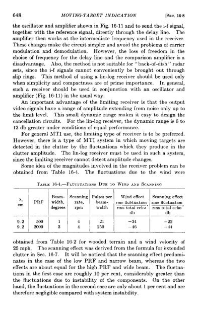
- Page 638 and 639: 638 MOVING TARGET INDICATION [SEC.
- Page 640 and 641: 640 MOVING TARGET INDICATION [SEC.
- Page 642 and 643: 642 MOVING-TARGET INDICATION [SEC.
- Page 644 and 645: 644 MOVING-TARGET INDICATION [SEC.
- Page 646 and 647: . 646 MOVING- TARGET INDICATION [SE
- Page 650 and 651: 650 MOVING-TARGET INDICATION [SEC.
- Page 652 and 653: 652 MOVING-TARGET INDICATION [SEC 1
- Page 654 and 655: 654 MOVING-TARGET INDICATION [SEC.
- Page 656 and 657: 656 MOVING-TARGET INDICATION [SEC.1
- Page 658 and 659: 658 When o = Othe instead MOVING-TA
- Page 660 and 661: 660 MOVING-TARGET INDICATION [SEC.
- Page 662 and 663: 662 MOVING TARGET INDICATION [SEC.1
- Page 664 and 665: 664 MOVING-TARGET INDICATION [SEC.
- Page 666 and 667: 666 MOVING-TARGET INDICATION [SEC.
- Page 668 and 669: 668 MOVING TARGET INDICATION [SEC.
- Page 670 and 671: 670 MO VINGTARGET INDICATION [SEC.
- Page 672 and 673: 672 MOVING TARGET INDICATION [SEC.1
- Page 674 and 675: 674 MOVING- TARGET INDICATION [SEC.
- Page 676 and 677: 676 MOVING-TARGET INDICATION ~SEC.
- Page 678 and 679: 678 MOVING-TARGET INDICATION [SEC.
- Page 680 and 681: CHAPTER 17 RADAR RELAY BY L. J. HAW
- Page 682 and 683: 682 RADAR RELAY [SEC. 172 transmitt
- Page 684 and 685: 684 RADAR RELAY [SEC. 17.3 staggeri
- Page 686 and 687: 686 RADAR RELAY [SEC. 17.4 excluded
- Page 688 and 689: 688 RADAR RELAY [SEC. 174 long sign
- Page 690 and 691: h Video I 1 I Angle marks RADAR REL
- Page 692 and 693: 692 [SEC. 175 ḇ 1 1 1 I ~ LKal tr
- Page 694 and 695: 694 RADAR RELAY [SEC. 17.5 generato
- Page 696 and 697: 696 RADAR RELAY [SEC. 17.6 station
- Page 698 and 699:
698 RADAR RELAY [SEC. 17.6 Video si
- Page 700 and 701:
700 RADAR RELAY [SEC. 176 train. Th
- Page 702 and 703:
702 RADAR RELAY [SEC.17.7 be obtain
- Page 704 and 705:
704 RADAR RELAY @EC. 17.7 illustrat
- Page 706 and 707:
[11 1 Bas,c pulse I %e pulse i ~--.
- Page 708 and 709:
708 RADAR ltELA Y [SEC. 1743 wave f
- Page 710 and 711:
710 RADAR RELAY [SEC. 17.8 actual m
- Page 712 and 713:
. 712 RADAR RELAY [SEC. 17.9 Such a
- Page 714 and 715:
714 RADAR RELAY [SEC. 17.10 between
- Page 716 and 717:
716 RADAR RELAY [SEC. 17.10 signal
- Page 718 and 719:
718 RADAR RELAY [SEC. 17.11 suppres
- Page 720 and 721:
720 RADAR RELAY [SEC. 17.12 provide
- Page 722 and 723:
722 RADAR RELAY [SEC. 17.13 relay l
- Page 724 and 725:
724 RADAR RELAY [SEC. 17.14 TaLE 17
- Page 726 and 727:
726 RADAR RELAY [SEC. 17.15 RADAR R
- Page 728 and 729:
728 RADAR RELAY [SEC. 17.15 Modulat
- Page 730 and 731:
730 RADAR RELAY [SEC. 17.15 the sec
- Page 732 and 733:
732 RADAR RELAY [SEC. 17.10 pulses
- Page 734 and 735:
734 RADAR RELAY [f+iEc.17.16 The vi
- Page 737 and 738:
Index A Absorbent materials, 69 Abs
- Page 739 and 740:
INDEX 739 B-scope, electrostatic, 5
- Page 741 and 742:
INDEX 741 Fairbank, W. M.,80 F Fan
- Page 743 and 744:
INDEX ’743 Microwave, reason for
- Page 745 and 746:
INDEX 745 Radar, pulse,3 range perf
- Page 747 and 748:
INDEX 747 Signal, interference of,