- Page 2 and 3:
Pile Design and Construction Practi
- Page 4 and 5:
Pile Design and Construction Practi
- Page 6 and 7:
Contents Preface to fifth edition i
- Page 8 and 9:
7.3 Designing piles to resist drivi
- Page 10 and 11:
Preface to fifth edition Piling rig
- Page 12:
Preface to fifth edition xi Pearson
- Page 16 and 17:
Chapter 1 General principles and pr
- Page 18 and 19:
(a) Backfill Bulb of pressure Appli
- Page 20 and 21:
are allowed to be used by Eurocode
- Page 22 and 23:
application of different load facto
- Page 24 and 25:
Load transfer The contractor’s gu
- Page 26 and 27:
(7) Jacked-down steel tube with clo
- Page 28 and 29:
Types of pile 13 needed to avoid cr
- Page 30 and 31:
(a) (b) Precast concrete Head of ti
- Page 32 and 33:
Table 2.2 Modification factor K 2 b
- Page 34 and 35:
4d d 10 mm M.S. plate sleeve tarred
- Page 36 and 37:
Table 2.3 Working loads and maximum
- Page 38 and 39:
Cement content �300 kg/m3 �325
- Page 40 and 41:
Types of pile 25 Table 2.5 BS 8004
- Page 42 and 43:
(a) (b) (c) (d) Cast iron or cast s
- Page 44 and 45:
Sheathing Bottom boards Figure 2.9
- Page 46 and 47:
Misplaced bearers Lifting holes Cra
- Page 48 and 49:
Section Bayonet plug Plan Locking p
- Page 50 and 51:
Existing foundation Precast pile ca
- Page 52 and 53:
Types of pile 37 Where very long le
- Page 54 and 55:
Types of pile 39 rotate during driv
- Page 56 and 57:
Types of pile 41 Because of their r
- Page 58 and 59:
(a) (b) Types of pile 43 Figure 2.2
- Page 60 and 61:
(a) (b) Welds Welds Types of pile 4
- Page 62 and 63:
(a) M.S. plate shoe Welds (b) 2.2.6
- Page 64 and 65:
Types of pile 49 brittle fracture r
- Page 66 and 67:
(a) (b) (c) Hammer Driving tube Con
- Page 68 and 69:
Types of pile 53 all cast-in-place
- Page 70 and 71:
Figure 2.28 The TaperTube pile.
- Page 72 and 73:
(a) (b) Figure 2.29 (a) The ScrewSo
- Page 74 and 75:
Types of pile 59 The simplest form
- Page 76 and 77:
Types of pile 61 Transverse reinfor
- Page 78 and 79:
Types of pile 63 completion the res
- Page 80 and 81:
Types of pile 65 permanently in the
- Page 82 and 83:
Types of pile 67 (3) Construction o
- Page 84 and 85:
Types of pile 69 can withstand fair
- Page 86 and 87:
Chapter 3 Piling equipment and meth
- Page 88 and 89:
Piling equipment and methods 73 A r
- Page 90 and 91:
Maximum height 26.32 m Usable leade
- Page 92 and 93:
Figure 3.4 Liebherr LRH 400 48 m lo
- Page 94 and 95:
Piling equipment and methods 79 the
- Page 96 and 97:
Piling frame Single-acting hammer S
- Page 98 and 99:
Guides for engaging leaders Steam o
- Page 100 and 101:
Table 3.1 Characteristics of some s
- Page 102 and 103:
Table 3.2 Characteristics of some h
- Page 104 and 105:
Piling equipment and methods 89 Tab
- Page 106 and 107:
Table 3.4 Characteristics of some d
- Page 108 and 109:
Figure 3.16 Driving a pile casing w
- Page 110 and 111:
Table 3.5 Continued Piling equipmen
- Page 112 and 113:
Soil resistance to driving (MN) 25
- Page 114 and 115:
Figure 3.19 Noise-abatement tower u
- Page 116 and 117:
Dolly M.S. plate Plastics Hardwood
- Page 118 and 119:
Standard elbow bend Detachable scre
- Page 120 and 121:
Figure 3.24 Discharging concrete in
- Page 122 and 123:
Piling equipment and methods 107 Fi
- Page 124 and 125:
Piling equipment and methods 109 Fi
- Page 126 and 127:
Table 3.6 Continued Piling equipmen
- Page 128 and 129:
Figure 3.30 Top-hinged under-reamin
- Page 130 and 131:
Piling equipment and methods 115 Fi
- Page 132 and 133:
Rotary table Hydraulic motor Water
- Page 134 and 135:
Piling equipment and methods 119 Fi
- Page 136 and 137:
Piling equipment and methods 121 sl
- Page 138 and 139:
Pile head Pile base 2 holes ∅ 4 m
- Page 140 and 141:
Piling equipment and methods 125 Ca
- Page 142 and 143:
Piling equipment and methods 127 sm
- Page 144 and 145:
Piling equipment and methods 129 Fi
- Page 146 and 147:
Piling equipment and methods 131 Th
- Page 148 and 149:
Piling equipment and methods 133 th
- Page 150 and 151:
Piling equipment and methods 135 Pi
- Page 152 and 153:
Piling equipment and methods 137 ve
- Page 154 and 155:
Chapter 4 Calculating the resistanc
- Page 156 and 157:
O C Settlement A Reloading Load B U
- Page 158 and 159:
Resistance of piles to compressive
- Page 160 and 161:
for spread foundations in various c
- Page 162 and 163:
Resistance of piles to compressive
- Page 164 and 165:
structural actions and A2 to geotec
- Page 166 and 167:
Geometrical data are concerned with
- Page 168 and 169:
Figure 4.3 Failure surfaces for com
- Page 170 and 171:
Depth below ground level in m 5.6 1
- Page 172 and 173:
(a) (b) Peak adhesion factor a p Le
- Page 174 and 175:
orehole or test profile over the pe
- Page 176 and 177:
Resistance of piles to compressive
- Page 178 and 179:
Effective length Shaft friction not
- Page 180 and 181:
4.3 Piles in coarse-grained soils 4
- Page 182 and 183:
Depth below ground surface (m) Resi
- Page 184 and 185:
Depth of penetration (m) 0 0 5 10 1
- Page 186 and 187:
using standard penetration tests or
- Page 188 and 189:
� � Resistance of piles to comp
- Page 190 and 191:
Resistance of piles to compressive
- Page 192 and 193:
Resistance of piles to compressive
- Page 194 and 195:
Safety factors generally used in th
- Page 196 and 197:
Depth to NAP datum (m) Cone resista
- Page 198 and 199:
The conditions at the interface can
- Page 200 and 201:
The shear modulus G in equation 4.3
- Page 202 and 203:
Resistance of piles to compressive
- Page 204 and 205:
2.0 OD tubular steel pile with clos
- Page 206 and 207:
where Resistance of piles to compre
- Page 208 and 209:
eached the point of ultimate resist
- Page 210 and 211:
(4) Obtain the safe end-bearing loa
- Page 212 and 213:
Vertical force, t t-z curve Vertica
- Page 214 and 215:
where the bearing capacity factor:
- Page 216 and 217:
and RQD of the rock as shown in Tab
- Page 218 and 219:
Depth below ground level (m) 0 5 10
- Page 220 and 221:
settlement of the pile are summariz
- Page 222 and 223:
Rock socket reduction factor a 1.0
- Page 224 and 225:
Table 4.17 � and � values of we
- Page 226 and 227:
Resistance of piles to compressive
- Page 228 and 229:
Influence factor, l p 2.0 1.6 1.2 0
- Page 230 and 231:
(a) (b) No load on pile head Residu
- Page 232 and 233:
Resistance of piles to compressive
- Page 234 and 235:
Resistance of piles to compressive
- Page 236 and 237:
Resistance of piles to compressive
- Page 238 and 239:
Resistance of piles to compressive
- Page 240 and 241:
a closed end into a deep deposit of
- Page 242 and 243:
Average shearing strength along pil
- Page 244 and 245:
It is assumed that the shear streng
- Page 246 and 247:
Depth below ground level (m) Figure
- Page 248 and 249:
Figure 4.45 Depth below ground leve
- Page 250 and 251:
Depth of h(m) Segment (m bql) � h
- Page 252 and 253:
For a wall thickness of 19 mm in mi
- Page 254 and 255:
Resistance of piles to compressive
- Page 256 and 257:
Pile groups under compressive loadi
- Page 258 and 259:
24.0 m 16.0 m The comparative group
- Page 260 and 261:
where c � cohesion intercept of s
- Page 262 and 263:
Inclination factor, i c Inclination
- Page 264 and 265:
Pile groups under compressive loadi
- Page 266 and 267:
z/B 0 0 0.1 0.2 0.3 0.4 0.5 0.6 0.7
- Page 268 and 269:
Compressive stress 1.5 q n q n B A
- Page 270 and 271:
E u/c u 3000 2500 2000 1500 1000 50
- Page 272 and 273:
0 0 1 2 3 4 H/B 5 6 7 8 9 0 1 2 3 4
- Page 274 and 275:
Pile groups under compressive loadi
- Page 276 and 277:
D LB LB D 0.50 0 0.1 0.2 0.3 0.4 0.
- Page 278 and 279:
Pile groups under compressive loadi
- Page 280 and 281:
Pile groups under compressive loadi
- Page 282 and 283:
Pile groups under compressive loadi
- Page 284 and 285:
Initial tangent constrained modulus
- Page 286 and 287:
factor N for which Schmertmann sugg
- Page 288 and 289:
Pile groups under compressive loadi
- Page 290 and 291:
0 0 2 4 H/B 6 8 10 Influence factor
- Page 292 and 293:
Pile groups under compressive loadi
- Page 294 and 295:
Overall loading 100 kN/m2 (a) (b) (
- Page 296 and 297:
Pile groups under compressive loadi
- Page 298 and 299:
(a) (b) (c) (d) Pile groups under c
- Page 300 and 301:
Pile groups under compressive loadi
- Page 302 and 303:
Pile groups under compressive loadi
- Page 304 and 305:
Pile groups under compressive loadi
- Page 306 and 307:
Depth below ground level in m 5 10
- Page 308 and 309:
For the arrangement of the piles sh
- Page 310 and 311:
Pile groups under compressive loadi
- Page 312 and 313:
Soft clay Sand B/2 5 11.2 m Figure
- Page 314 and 315: Pile groups under compressive loadi
- Page 316 and 317: Unit negative skin friction at top
- Page 318 and 319: Pile groups under compressive loadi
- Page 320 and 321: Chapter 6 The design of piled found
- Page 322 and 323: (a) Tie rod Wholly compression Whol
- Page 324 and 325: esistance of cylindrical augered fo
- Page 326 and 327: in the ground is assumed to be equa
- Page 328 and 329: Section 3.3.1. Enlargements cannot
- Page 330 and 331: Piles to resist uplift and lateral
- Page 332 and 333: Spacer Top of hard rock Drilling pi
- Page 334 and 335: where m is the modular ratio of ste
- Page 336 and 337: Table 6.3 Examples of bond stress b
- Page 338 and 339: Top of rock 30˚ 30˚ Figure 6.15 F
- Page 340 and 341: (b) P/n & �Vm Vc 2.0 1.8 1.6 1.4
- Page 342 and 343: Table 6.4 Partial resistance factor
- Page 344 and 345: and adjustment, starting with a ver
- Page 346 and 347: Coefficient of subgrade modulus var
- Page 348 and 349: where e is the height from the grou
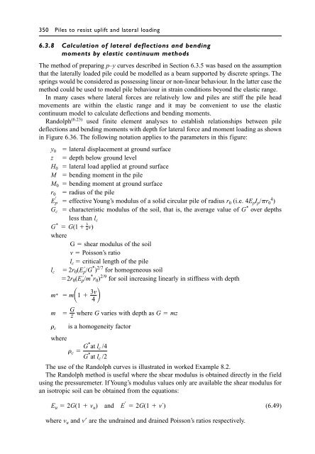
- Page 350 and 351: and Thus from Figure 6.24 deflectio
- Page 352 and 353: (a) Deflection coefficient Ay (c) D
- Page 354 and 355: (a) (b) (c) Depth coefficient Z 0 1
- Page 356 and 357: Horizontal load H; Bending moment =
- Page 358 and 359: Methods of drawing sets of p-y curv
- Page 360 and 361: Calculations to determine the ultim
- Page 362 and 363: (a) (b) Pressure Soil reaction p Ps
- Page 366 and 367: (a) yroGc H0 Ep Gc 1/7 (b) 0 0 0.1
- Page 368 and 369: (a) determining the compressive and
- Page 370 and 371: A X Z B R A Resultant R R B Y C D R
- Page 372 and 373: 6.8 FREEMAN, C. F., KLAJNERMAN, D.,
- Page 374 and 375: Thus the load to be carried by anch
- Page 376 and 377: If high-tensile steel (which has a
- Page 378 and 379: sustained horizontal load which can
- Page 380 and 381: Calculating the allowable horizonta
- Page 382 and 383: Pile cap (Weight�2475 kN) F E D C
- Page 384 and 385: The resultant of the vertical and h
- Page 386 and 387: The Brinch Hansen bearing capacity
- Page 388 and 389: Modulus of elasticity of pile � 2
- Page 390 and 391: Chapter 7 Some aspects of the struc
- Page 392 and 393: (a) (b) (c) Lifting rope Lifting po
- Page 394 and 395: 7.3 Designing piles to resist drivi
- Page 396 and 397: Structural design of piles and pile
- Page 398 and 399: Structural design of piles and pile
- Page 400 and 401: should not arise if the piles are d
- Page 402 and 403: (a) (b) (c) M.S.plate cover M.S.cap
- Page 404 and 405: 45˚ Structural design of piles and
- Page 406 and 407: X Column Y9 Y9 Y Critical section f
- Page 408 and 409: 7.9 The design of pile capping beam
- Page 410 and 411: Damp-proof course Cranked vent Grou
- Page 412 and 413: Structural design of piles and pile
- Page 414 and 415:
(a) (b) Deck of wharf Fender Rubber
- Page 416 and 417:
(a) (b) y y e z f A The bending mom
- Page 418 and 419:
Piling for marine structures 403 th
- Page 420 and 421:
Pipe trunkways Hose handling platfo
- Page 422 and 423:
Piling for marine structures 407 8.
- Page 424 and 425:
Piling for marine structures 409 sh
- Page 426 and 427:
In SI units, equation 8.8 becomes f
- Page 428 and 429:
The natural frequency of the member
- Page 430 and 431:
The empirical equation of Korzhavin
- Page 432 and 433:
Piling for marine structures 417 re
- Page 434 and 435:
Table 8.3 Minimum safety factors fo
- Page 436 and 437:
Piling for marine structures 421 th
- Page 438 and 439:
Piling for marine structures 423 sh
- Page 440 and 441:
8.21 GERWICK, B. C. Construction of
- Page 442 and 443:
Soil resistance p in kN per m of de
- Page 444 and 445:
From Figures 6.29a and b the comput
- Page 446 and 447:
giving 9.7y � 0.26, y � 0.26
- Page 448 and 449:
From �7.5 to �3.0 m: no increas
- Page 450 and 451:
Miscellaneous piling problems 435 W
- Page 452 and 453:
9.2 Piling for underpinning Miscell
- Page 454 and 455:
Miscellaneous piling problems 439 B
- Page 456 and 457:
Miscellaneous piling problems 441 T
- Page 458 and 459:
Miscellaneous piling problems 443 p
- Page 460 and 461:
Longitudinal reinforcement is provi
- Page 462 and 463:
Light-gauge steel lining tubes Stow
- Page 464 and 465:
When inspecting the geological cond
- Page 466 and 467:
Miscellaneous piling problems 451 f
- Page 468 and 469:
natural ‘freeze-back’ around th
- Page 470 and 471:
Miscellaneous piling problems 455 b
- Page 472 and 473:
Miscellaneous piling problems 457 w
- Page 474 and 475:
Drainage layer 8.0 m 6.0 m Fill 1.0
- Page 476 and 477:
p m/c u 10.5 2p 0 and the mean hori
- Page 478 and 479:
Bridge abutment support piles Emban
- Page 480 and 481:
Figure 9.23 Drilling equipment for
- Page 482 and 483:
Max. water level +16 m Min. water l
- Page 484 and 485:
2-4 m marine clay dredged out MHW R
- Page 486 and 487:
Miscellaneous piling problems 471 o
- Page 488 and 489:
Miscellaneous piling problems 473 c
- Page 490 and 491:
The ground temperature around the p
- Page 492 and 493:
9.40 URANOWSKI, D. D., DODDS, S., a
- Page 494 and 495:
The durability of piled foundations
- Page 496 and 497:
and European Standards as shown in
- Page 498 and 499:
The durability of piled foundations
- Page 500 and 501:
martesia with some teredo, and at C
- Page 502 and 503:
The durability of piled foundations
- Page 504 and 505:
The durability of piled foundations
- Page 506 and 507:
The durability of piled foundations
- Page 508 and 509:
The durability of piled foundations
- Page 510 and 511:
The durability of piled foundations
- Page 512 and 513:
economics, taking into account the
- Page 514 and 515:
Depth of borehole 1.5 B 1 in 4 B Gr
- Page 516 and 517:
Ground investigations, contracts an
- Page 518 and 519:
Ground investigations, contracts an
- Page 520 and 521:
(a) DCP n (blows/100 mm) 40 35 30 2
- Page 522 and 523:
Ground investigations, contracts an
- Page 524 and 525:
Ground investigations, contracts an
- Page 526 and 527:
Ground investigations, contracts an
- Page 528 and 529:
Ground investigations, contracts an
- Page 530 and 531:
Table 11.2 Daily pile record for dr
- Page 532 and 533:
Paper fixed to pile by adhesive tap
- Page 534 and 535:
Ground investigations, contracts an
- Page 536 and 537:
Ground investigations, contracts an
- Page 538 and 539:
Ground investigations, contracts an
- Page 540 and 541:
Figure 11.10 Patented arrangement f
- Page 542 and 543:
following expressions: (11.1) Load
- Page 544 and 545:
(b) Settlement of pile head in mm S
- Page 546 and 547:
(a) Settlement � (mm) 0 0 4 8 Gro
- Page 548 and 549:
Ground investigations, contracts an
- Page 550 and 551:
Ground investigations, contracts an
- Page 552 and 553:
experience to give reasonably relia
- Page 554 and 555:
Appendix Properties of materials A.
- Page 556:
Subdivisions of Grades A to C chalk
- Page 559 and 560:
544 Name index Davis, E. H. 354 Dav
- Page 561 and 562:
546 Name index Schaaf, S. A. 424 Sc
- Page 563 and 564:
548 Subject index contiguous piles
- Page 565 and 566:
550 Subject index Pali Radice piles