- Page 3 and 4: Digital Video and HDTV Algorithms a
- Page 5 and 6: Publishing Director: Diane Cerra Pu
- Page 7 and 8: Digital Video and HDTV Algorithms a
- Page 10 and 11: Raster images 1 This chapter introd
- Page 12 and 13: 4:3 16:9 Figure 1.3 Pan-and-scan cr
- Page 14 and 15: Figure 1.7 Pixel arrays of several
- Page 16 and 17: SDTV 1’ ( 1⁄60°) d= 1⁄480 SD
- Page 18 and 19: See Appendix B, Introduction to rad
- Page 20 and 21: 4095 101 100 0 ∆ = 1% 40.95 : 1 F
- Page 22 and 23: See Bit depth requirements, on page
- Page 24 and 25: Resolution properly refers to spati
- Page 26 and 27: The oct in octave refers to the eig
- Page 28 and 29: Sound pressure level, relative 1 0
- Page 30 and 31: Figure 2.4 Footroom and headroom ar
- Page 32 and 33: Figure 3.1 Contrast control determi
- Page 34 and 35: SMPTE RP 71, Setting Chromaticity a
- Page 36 and 37: Figure 3.7 Brightness control in Ph
- Page 38 and 39: Raster images in computing 4 This c
- Page 40 and 41: Symbolic image description Many met
- Page 42 and 43: Grayscale A grayscale image represe
- Page 44 and 45: Poynton, Charles, “The rehabilita
- Page 46 and 47: The browser-safe palette forms a ra
- Page 48 and 49: Image width is the product of socal
- Page 52 and 53: Figure 5.3 Diagonal line reconstruc
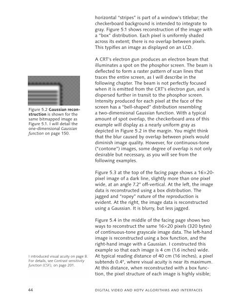
- Page 54 and 55: Figure 5.7 Bitmapped graphic image,
- Page 56 and 57: Figure 5.8 Gaussian spot size. Soli
- Page 58 and 59: Flicker is sometimes redundantly ca
- Page 60 and 61: The word raster is derived from the
- Page 62 and 63: Figure 6.3 Production aperture comp
- Page 64 and 65: TEST SCENE SCANNING FIRST FIELD Ima
- Page 66 and 67: Progressive Interlaced Image row 0
- Page 68 and 69: FIRST FIELD SECOND FIELD Figure 6.1
- Page 70 and 71: Table 6.3 Video systems are classif
- Page 72 and 73: An electrical engineer may call thi
- Page 74 and 75: When digital information is process
- Page 76 and 77: Resolution properly refers to spati
- Page 78 and 79: Figure 7.6 Vertical resolution in 4
- Page 80 and 81: Pixel count places a constraint on
- Page 82 and 83: The term luminance is widely misuse
- Page 84 and 85: Figure 8.4 Nonlinearly coded relati
- Page 86 and 87: Tristimulus values are correctly re
- Page 88 and 89: Giorgianni, Edward J., and T.E. Mad
- Page 90 and 91: Simultaneous contrast ratio is the
- Page 92 and 93: Imaging system Some people suggest
- Page 94 and 95: Introduction to luma and chroma 10
- Page 96 and 97: Luma and color differences can be c
- Page 98 and 99: 4:2:0 This scheme is used in JPEG/J
- Page 100 and 101:
Figure 10.4 Interstitial chroma fil
- Page 102 and 103:
The notation CCIR is often wrongly
- Page 104 and 105:
Square sampling Component 4:2:2 Rec
- Page 106 and 107:
Component 4:2:2 Rec. 601-5 The tech
- Page 108 and 109:
See Table 13.1, on page 114, and th
- Page 110 and 111:
NTSC stands for National Television
- Page 112 and 113:
NTSC and PAL encoding NTSC or PAL e
- Page 114 and 115:
Figure 12.2 S-video interface invol
- Page 116:
Concerning the absence of D-4 in th
- Page 119 and 120:
Figure 13.1 Comparison of aspect ra
- Page 121 and 122:
ATSC A/53, Digital Television Stand
- Page 123 and 124:
System Scanning SMPTE standard STL
- Page 125 and 126:
data stored in scan-line order, hor
- Page 127 and 128:
Compression ratio Quality/applicati
- Page 129 and 130:
Figure 14.2 MPEG group of pictures
- Page 131 and 132:
Figure 14.6 Example GOP I0B1B2P3B4B
- Page 133 and 134:
Many MPEG terms - such as frame, pi
- Page 135 and 136:
Voltage, mV 700 350 0 -300 Code, 8-
- Page 137 and 138:
SMPTE 259M, 10-Bit 4:2:2 Component
- Page 139 and 140:
Voltage, mV 700 350 SMPTE 305.2M, S
- Page 141 and 142:
IEC 61883-1, Consumer audio/video e
- Page 143 and 144:
For details concerning SCH, see pag
- Page 145 and 146:
Some video switchers incorporate di
- Page 148 and 149:
My explanation describes the origin
- Page 150 and 151:
Figure 16.2 Cosine waves at exactly
- Page 152 and 153:
1 1+ sin 0.75 ωt 2 0.5 Figure 16.6
- Page 154 and 155:
0 1 2 3 1.0 0.8 0.6 0.4 0.2 0 Time,
- Page 156 and 157:
-5 -4 -3 -2 1.0 0.8 0.6 0.4 0.2 -1
- Page 158 and 159:
Impulse (point sampling) 0 1 t 0 2
- Page 160 and 161:
Figure 16.12 [1, 1] FIR filter sums
- Page 162 and 163:
Figure 16.17 5-tap FIR filter respo
- Page 164 and 165:
Figure 16.20 Comb filter response r
- Page 166 and 167:
125 ns, 45° at 1 MHz 125 ns, 90°
- Page 168 and 169:
Compensation of undesired phase res
- Page 170 and 171:
ωS 2 ⎛ 1 ⎞ Eq 16.3 Ne ≈ ⋅
- Page 172 and 173:
We could use the term weighting, bu
- Page 174 and 175:
Figure 16.26 FIR filter example, 25
- Page 176 and 177:
1 1+ sin 0.44 ωt 2 0.5 Figure 16.2
- Page 178 and 179:
Resampling, interpolation, and deci
- Page 180 and 181:
Figure 17.1 Two-times upsampling st
- Page 182 and 183:
Figure 17.4 Analog filter for direc
- Page 184 and 185:
Julius O. Smith calls this Waring-
- Page 186 and 187:
Smith, A.R., “Planar 2-pass textu
- Page 188 and 189:
You can consider the entire stopban
- Page 190 and 191:
1 1 1 512 2 2 8 = · In a direct im
- Page 192:
Taken literally, decimation involve
- Page 195 and 196:
0 Horizontal displacement (fraction
- Page 197 and 198:
Figure 18.7 Spatial frequency spect
- Page 199 and 200:
Schreiber, William F., and Donald E
- Page 201 and 202:
Oversampling to double the number o
- Page 203 and 204:
10 k 1 k 100 10 1 100 m 10 m 100 1
- Page 205 and 206:
Viewing environment Max. luminance,
- Page 207 and 208:
ISO 5-1, Photography - Density meas
- Page 209 and 210:
Campbell, F.W., and V.G. Robson,
- Page 211 and 212:
See Introduction to radiometry and
- Page 213 and 214:
SMPTE RP 71, Setting Chromaticity a
- Page 215 and 216:
Figure 20.2 Luminance and lightness
- Page 218 and 219:
Figure 21.1 Example coordinate syst
- Page 220 and 221:
Power, relative 400 500 600 700 Wav
- Page 222 and 223:
B G 400 500 600 700 400 500 600 700
- Page 224 and 225:
The term sharpening is used in the
- Page 226 and 227:
Grassmann’s Third Law: Sources of
- Page 228 and 229:
1 y = 1- x 1 Spectral locus Line of
- Page 230 and 231:
Figure 21.9 SPDs of blackbody radia
- Page 232 and 233:
Tungsten illumination can’t have
- Page 234 and 235:
∆E* is pronounced DELTA E-star. i
- Page 236 and 237:
McCamy argues that under normal con
- Page 238:
Wyszecki, Günter, and W.S. Styles,
- Page 241 and 242:
If you are unfamiliar with the term
- Page 243 and 244:
CIE standards established in 1964 w
- Page 245 and 246:
Table 22.2 NTSC primaries (obsolete
- Page 247 and 248:
IEC FDIS 61966-2-1, Multimedia syst
- Page 249 and 250:
Michael Brill and R.W.G. Hunt argue
- Page 251 and 252:
CMF of X sensor CMF of Y sensor CMF
- Page 253 and 254:
CMF of Red sensor CMF of Green sens
- Page 255 and 256:
Spectral sensitivity of Red sensor
- Page 257 and 258:
For the D 65 reference now standard
- Page 259 and 260:
Eq 22.10 RGB components where one o
- Page 261 and 262:
SMPTE RP 71, Setting Chromaticity a
- Page 263 and 264:
Poynton, Charles, “Wide Gamut Dev
- Page 265 and 266:
Opto-electronic transfer function (
- Page 267 and 268:
Roberts, Alan, “Measurement of di
- Page 269 and 270:
The importance of rendering intent,
- Page 271 and 272:
See Headroom and footroom, on page
- Page 273 and 274:
Eq 23.7 Video signal, V’ 1.2 1.0
- Page 275 and 276:
Figure 23.5 Rec. 709, sRGB, and CIE
- Page 277 and 278:
PDP and DLP devices are commonly de
- Page 279 and 280:
Concerning the conversion between R
- Page 281 and 282:
Video, PC TRISTIM. Computergenerate
- Page 283 and 284:
An SGI workstation can be set to ha
- Page 285 and 286:
The Rec. 709 function is suitable f
- Page 287 and 288:
What are loosely called JPEG files
- Page 289 and 290:
+1 G AXIS 0 G Bk 0 255 G’ COMPONE
- Page 291 and 292:
Here the term color difference refe
- Page 293 and 294:
Figure 24.3 shows a time delay elem
- Page 295 and 296:
See Appendix A, YUV and luminance c
- Page 297 and 298:
Nonlinear red, green, blue (R’G
- Page 299 and 300:
The mismatch between the primaries
- Page 301 and 302:
XYZ or R 1G 1B 1 TRISTIMULUS 3×3 (
- Page 303 and 304:
Owing to the dependence of the opti
- Page 305 and 306:
Luma/color difference component set
- Page 307 and 308:
System Notation Color difference sc
- Page 309 and 310:
For a discussion of primary chromat
- Page 311 and 312:
Figure 25.2 P BP R components for S
- Page 313 and 314:
The Y’P B P R and Y’C B C R sca
- Page 315 and 316:
Eq 25.6 Eq 25.7 You can determine t
- Page 317 and 318:
+128 +127 0 -128 (clipped) 0 Figure
- Page 319 and 320:
When the term Y’UV (or YUV) is en
- Page 321 and 322:
Yl G G Figure 26.1 B’-Y’, R’-
- Page 323 and 324:
Figure 26.3 CBCR compo- +112 nents
- Page 325 and 326:
Concerning Pointer, see the margina
- Page 327 and 328:
Equations 26.12 and 26.13 are writt
- Page 330 and 331:
100% 90% 50% 10% 0% 0 1 2 3 4 5 Y
- Page 332 and 333:
Active lines (vertically) encompass
- Page 334 and 335:
Back porch is described in Analog h
- Page 336 and 337:
255 Full-range code, computing 0 -1
- Page 338 and 339:
danger in using such operations: Up
- Page 340 and 341:
If you use CTI, you run the risk of
- Page 342 and 343:
See Appendix A, YUV and luminance c
- Page 344 and 345:
Eq 28.3 Eq 28.4 Eq 28.5 Eq 28.6 1
- Page 346 and 347:
It is unfortunate that the formulat
- Page 348 and 349:
COMPOSITE NTSC VIDEO Y’/C SEPARAT
- Page 350 and 351:
COMPOSITE PAL VIDEO Y’/C SEPARATO
- Page 352 and 353:
COMPOSITE VIDEO or S-video LUMA COM
- Page 354:
COMPOSITE NTSC VIDEO Saturation Hue
- Page 357 and 358:
Y’ C f SC Figure 29.1 Y’/C spec
- Page 359 and 360:
1 2 ... 262 263 Figure 29.4 Color s
- Page 361 and 362:
Figure 29.7 Dot crawl is exhibited
- Page 363 and 364:
1 2 3 4 ... Figure 29.9 Color subca
- Page 365 and 366:
COMPOSITE PAL VIDEO Y’/C SEPARATO
- Page 367 and 368:
t Opposite field Y’+C t+1⁄59.94
- Page 369 and 370:
CHROMA FILTER RESPONSE CHROMA (C) S
- Page 371 and 372:
CHROMA (C) SPECTRAL POWER LUMA (Y
- Page 373 and 374:
Because an analog demodulator canno
- Page 375 and 376:
Y’ I Q 1.3 MHz 600 kHz SUBCARRIER
- Page 377 and 378:
A decoder cannot determine whether
- Page 379 and 380:
525 · 60 = 15750 2 Line rate The t
- Page 381 and 382:
60 1000 525× 2 1001 315 88 3 57954
- Page 383 and 384:
Sampling NTSC at 4f SC gives 910 sa
- Page 385 and 386:
60 Hz 7 · 5 · 5 · 3 525/60 (480
- Page 387 and 388:
3· 588· 25 Hz = 44100 Hz 3 490 30
- Page 389 and 390:
See Frame, field, line, and sample
- Page 391 and 392:
SMPTE 258M, Television - Transfer o
- Page 393 and 394:
The IRE unit is introduced on page
- Page 395 and 396:
SMPTE 12M, Time and Control Code. S
- Page 397 and 398:
The V and H bits are asserted durin
- Page 399 and 400:
* 1250/50 is an exception; see SMPT
- Page 401 and 402:
See NTSC two-frame sequence, on pag
- Page 403 and 404:
SMPTE 260M describes a scheme, now
- Page 405 and 406:
SMPTE 292M, Bit-Serial Digital Inte
- Page 407 and 408:
A Naive combined sync establishes h
- Page 409 and 410:
1 PRE- BROAD EQUALIZATION PULSES 0V
- Page 411 and 412:
Most lines have a single normalwidt
- Page 413 and 414:
1 23 4 5 6 7 Figure 34.6 Sync separ
- Page 415 and 416:
Figure 34.7 BNC connector Figure 34
- Page 418 and 419:
Figure 35.1 A videotape recorder (V
- Page 420 and 421:
In consumer VCR search mode playbac
- Page 422 and 423:
Heads for other longitudinal tracks
- Page 424 and 425:
The term sync in sync block is unre
- Page 426 and 427:
Notation Component analog VTRs are
- Page 428 and 429:
Even if playback errors are so seve
- Page 430 and 431:
Notation Method Tape width (track p
- Page 432 and 433:
D-7 (DVCPRO), DVCAM runs twice the
- Page 434 and 435:
D-12 (DVCPRO HD) The DV standard wa
- Page 436 and 437:
Figure 36.1 “2-3 pulldown” refe
- Page 438 and 439:
Film is transferred to 576i25 video
- Page 440 and 441:
FILM A A VIDEO, 2-3 PULLDOWN A VIDE
- Page 442 and 443:
Native 24 Hz coding Traditionally,
- Page 444 and 445:
Figure 37.1 Test scene FIRST FIELD
- Page 446 and 447:
For a modest improvement over 2-tap
- Page 448 and 449:
Figure 37.13 Interstitial spatial f
- Page 450:
IN Figure 37.17 Cosited spatial fil
- Page 454 and 455:
ISO/IEC 10918, Information Technolo
- Page 456 and 457:
Figure 38.2 DCT concentrates image
- Page 458 and 459:
Eq 38.1 Owing to the eight-line-hig
- Page 460 and 461:
In MPEG-2, DC terms can be coded wi
- Page 462 and 463:
Figure 38.8 Zigzag scanning is used
- Page 464 and 465:
Figure 38.12 Compression ratio cont
- Page 466 and 467:
Hamilton, Eric, JPEG File Interchan
- Page 468 and 469:
Concerning DVC recording, see page
- Page 470 and 471:
356 357 358 359 Figure 39.2 Chroma
- Page 472 and 473:
CMs in a segment are denoted a thro
- Page 474 and 475:
For a more elaborate description, a
- Page 476 and 477:
DV HD HD stands for high definition
- Page 478:
IEC 61904, Video recording - Helica
- Page 481 and 482:
MPEG-2 specifies several algorithmi
- Page 483 and 484:
422P@ML allows 608 lines at 25 Hz f
- Page 485 and 486:
Figure 40.1 MPEG-2 frame picture co
- Page 487 and 488:
If horizontal size or vertical size
- Page 489 and 490:
A prediction region in an anchor fr
- Page 491 and 492:
Each nonintra macroblock in an inte
- Page 493 and 494:
Figure 40.4 Frame DCT type involves
- Page 495 and 496:
Distributed refresh does not guaran
- Page 497 and 498:
Whether an encoder actually searche
- Page 499 and 500:
Figure 40.9 Buffer occupancy in MPE
- Page 501 and 502:
Group of pictures (GOP header) the
- Page 503 and 504:
Gibson, Jerry D., Toby Berger, Tom
- Page 506 and 507:
f FR f H 30 = ≈ 29. 97 Hz 1. 001
- Page 508 and 509:
Concerning closed captions, see ANS
- Page 510 and 511:
CHAPTER 41 480 i COMPONENT VIDEO 50
- Page 512 and 513:
SMPTE RP 187, Center, Aspect Ratio
- Page 514 and 515:
8-bit code 235 125 1 / 2 16 Figure
- Page 516 and 517:
Voltage, mV 700 350 0 -300 0 H EIA/
- Page 518 and 519:
480i NTSC composite video 42 Althou
- Page 520 and 521:
Concerning the association of U wit
- Page 522 and 523:
IEC 60933-5 (1992-11) Interconnecti
- Page 524 and 525:
8-bit code 200 176.25 70.5 60 4 757
- Page 526 and 527:
Derived line rate is 15.625 kHz. It
- Page 528 and 529:
For details concerning VITC in 576i
- Page 530 and 531:
CHAPTER 43 576 i COMPONENT VIDEO 52
- Page 532 and 533:
SMPTE RP 187, Center, Aspect Ratio
- Page 534 and 535:
Code 235 125 1 / 2 16 Figure 43.2 5
- Page 536 and 537:
1135 4 1 + = 625 709379 2500 = 283.
- Page 538 and 539:
See NTSC Y’IQ system, on page 365
- Page 540 and 541:
8-bit code 211 137.5 64 EBU Tech. 3
- Page 542 and 543:
ANSI/EIA-189-A, Encoded Color Bar S
- Page 544 and 545:
Figure 45.3 NTSC- Encoded 100/0/75/
- Page 546 and 547:
ITU-R Rec. BT.471, Nomenclature and
- Page 548 and 549:
Figure 45.7 Modulated 5-step stair
- Page 550 and 551:
( ) PULSE T The risetime, from 10%
- Page 552:
Figure 45.12 FCC composite test sig
- Page 555 and 556:
tri Trilevel pulse BR Broad pulse T
- Page 557 and 558:
550 DIGITAL VIDEO AND HDTV ALGORITH
- Page 559 and 560:
Component digital 4:2:2 interface Y
- Page 561 and 562:
Passband insertion gain, dB Stopban
- Page 564 and 565:
SMPTE 274M, 1920 × 1080 Scanning a
- Page 566 and 567:
tri Trilevel pulse BR Broad pulse L
- Page 568 and 569:
Trilevel sync comprises a negative
- Page 570 and 571:
Vertical interval video lines do no
- Page 572 and 573:
RGB primary components Picture info
- Page 574:
mV +700 +350 +300 0 -300 -44 +44 0H
- Page 578 and 579:
ITU-R Rec. BT.470, Conventional tel
- Page 580 and 581:
PAL-D is ambiguous, referring eithe
- Page 582 and 583:
Bower, A.J., NICAM 728 - Digital Tw
- Page 584 and 585:
SECAM had an advantage during the 1
- Page 586 and 587:
Consumer analog NTSC and PAL 49 Con
- Page 588 and 589:
Macrovision is a proprietary, paten
- Page 590 and 591:
CENELEC EN 50049-1:1989 IEC 60933-1
- Page 592:
VHS trick mode playback A VHS VCR h
- Page 595 and 596:
NHK Science and Technical Research
- Page 597 and 598:
I and Q refer to in-phase and quadr
- Page 599 and 600:
Weiss, S. Merrill, Issues in Advanc
- Page 602 and 603:
YUV and luminance considered harmfu
- Page 604 and 605:
Pritchard, D.H., “U.S. Color Tele
- Page 606 and 607:
When I say NTSC and PAL, I refer to
- Page 608 and 609:
ANSI/IESNA RP-16, Nomenclature and
- Page 610 and 611:
Palmer, James M., “Getting Intens
- Page 612 and 613:
Differentiate w.r.t. AREA power, P
- Page 614:
Ashdown, Ian, Radiosity: A Programm
- Page 617 and 618:
50 Hz. Each film frame is scanned t
- Page 619 and 620:
601 See Rec. 601, on page 643. 625/
- Page 621 and 622:
B-picture In MPEG, a bidirectionall
- Page 623 and 624:
BT.601, BT.709 See Rec. 601 and Rec
- Page 625 and 626:
CIE luminance, CIE Y See Luminance.
- Page 627 and 628:
information rate of the color diffe
- Page 629 and 630:
Contrast 1. Contrast ratio; see bel
- Page 631 and 632:
D-10 A SMPTE-standard component SDT
- Page 633 and 634:
Drive (n.) A periodic pulse signal
- Page 635 and 636:
2. In traditional video usage, the
- Page 637 and 638:
G/PAL See PAL-B/G/H, on page 640. (
- Page 639 and 640:
4. User-accessible means to adjust
- Page 641 and 642:
K-factor, K-rating A numerical char
- Page 643 and 644:
Luma A video signal representative
- Page 645 and 646:
2. In a camera or scanner, the cond
- Page 647 and 648:
Offset sampling Obsolete scanning t
- Page 649 and 650:
numerical parameter having a value
- Page 651 and 652:
Rendering intent Encoding and subse
- Page 653 and 654:
which is a function of the distribu
- Page 655 and 656:
Standards conversion Conversion, in
- Page 657 and 658:
transmission; or to color differenc
- Page 659 and 660:
Y’/C629, Y’/C688 Y’C 1 C 2 Y
- Page 661 and 662:
177 Mb/s 129-130 18 MHz sampling ra
- Page 663 and 664:
ambient illumination (cont’d) in
- Page 665 and 666:
inary group flags (in timecode) 386
- Page 667 and 668:
chroma (cont’d) modulation 94, 10
- Page 669 and 670:
color (cont’d) difference coding
- Page 671 and 672:
CRC (cyclic redundancy check) in HD
- Page 673 and 674:
Dolby 589 dominance, field 430 dot
- Page 675 and 676:
factor interlace 68, 70 K 542 Kell
- Page 677 and 678:
framebuffer 7 framestore 7 France 9
- Page 679 and 680:
hue (cont’d) hue decoder control
- Page 681 and 682:
ITU-T fax 7, 118 former CCITT 118 H
- Page 683 and 684:
longitudinal timecode 382, 384 Look
- Page 685 and 686:
N N/PAL 96, 575-576 N10 see also PA
- Page 687 and 688:
Panasonic 509-510 Paraguay 576 pari
- Page 689 and 690:
pulse (cont’d) colorframe 404 equ
- Page 691 and 692:
RMS (root mean square) 19, 146 Robe
- Page 693 and 694:
(sin x)/x 147, 149 (graph) also kno
- Page 695 and 696:
SVM (scan-velocity modulation) 330,
- Page 697 and 698:
uniformity, perceptual 21 in DCT/JP
- Page 699 and 700:
widescreen 4 HDTV 112 SDTV 99 480i
- Page 701:
This book is set in the Syntax type