Agilent Spectrum Analysis Basics - Agilent Technologies

More documents

Recommendations

Info

Let’s assume that we have some idea of the characteristics of our signal, but we do not know its exact frequency. How do we determine which is the real signal? The image-shift process retunes the LO fundamental frequency by an amount equal to 2f IF /N. This causes the Nth harmonic to shift by 2f IF . If we are tuned to a real signal, its corresponding pair will now appear at the same position on screen that the real signal occupied in the first sweep. If we are tuned to another multiple pair created by some other incorrect harmonic, the signal will appear to shift in frequency on the display. The ESA spectrum analyzer shifts the LO on alternate sweeps, creating the two displays shown in Figures 7-17a and 7-17b. In Figure 7-17a, the real signal (the 14 – mixing product) is tuned to the center of the screen. Figure 7-17b shows how the image shift function moves the corresponding pair (the 14 + mixing product) to the center of the screen. Figure 7-17a. 14 – centered Figure 7-17b. 14 + centered Figure 7-17. Alternate sweeps taken with the image shift function Let’s examine the second method of signal identification, called image suppression. In this mode, two sweeps are taken using the MIN HOLD function, which saves the smaller value of each display point, or bucket, from the two sweeps. The first sweep is done using normal LO tuning values. The second sweep offsets the LO fundamental frequency by 2f IF /N. As we saw in the first signal ID method, the image product generated by the correct harmonic will land at the same point on the display as the real signal did on the first sweep. Therefore, the trace retains a high amplitude value. Any false response that shifts in frequency will have its trace data replaced by a lower value. Thus, all image and incorrect multiple responses will appear as noise. This is shown in Figure 7-18. 100
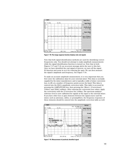
Figure 7-18. The image suppress function displays only real signals Note that both signal identification methods are used for identifying correct frequencies only. You should not attempt to make amplitude measurements while the signal identification function is turned on. Note that in both Figures 7-17 and 7-18, an on-screen message alerts the user to this fact. Once we have identified the real signal of interest, we turn off the signal ID function and zoom in on it by reducing the span. We can then measure the signal’s amplitude and frequency. See Figure 7-19. To make an accurate amplitude measurement, it is very important that you first enter the calibration data for your external mixer. This data is normally supplied by the mixer manufacturer, and is typically a table of mixer conversion loss, in dB, at a number of frequency points across the band. This data is entered into the ESA’s amplitude correction table. This table is accessed by pressing the [AMPLITUDE] key, then pressing the {More}, {Corrections}, {Other} and {Edit} softkeys. After entering the conversion loss values, apply the corrections with the {Correction On} softkey. The spectrum analyzer reference level is now calibrated for signals at the input to the external mixer. If you have other loss or gain elements between the signal source and the mixer, such as antennas, cables, or preamplifiers, the frequency responses of these elements should be entered into the amplitude correction table as well. Figure 7-19. Measurement of positively identified signal 101
Page 1 and 2:
Agilent Spectrum Analysis Basics Ap
Page 3 and 4:
Table of Contents — continued Cha
Page 5 and 6:
Some measurements require that we p
Page 7 and 8:
Figure 1-3. Harmonic distortion tes
Page 9 and 10:
While we have defined spectrum anal
Page 11 and 12:
Since the output of a spectrum anal
Page 13 and 14:
We need to pick an LO frequency and
Page 15 and 16:
To separate closely spaced signals
Page 17 and 18:
Agilent data sheets describe the ab
Page 19 and 20:
This allows us to calculate the fil
Page 21 and 22:
Some modern spectrum analyzers allo
Page 23 and 24:
On the other hand, the rise time of
Page 25 and 26:
The width of the resolution (IF) fi
Page 27 and 28:
The “bucket” concept is importa
Page 29 and 30:
Peak (positive) detection One way t
Page 31 and 32:
The normal detection algorithm: If
Page 33 and 34:
EMI detectors: average and quasi-pe
Page 35 and 36:
The effect is most noticeable in me
Page 37 and 38:
Thus, the display gradually converg
Page 39 and 40:
In some cases, time-gating capabili
Page 41 and 42:
Timeslots 0 1 2 3 4 5 6 7 Timeslots
Page 43 and 44:
Gated sweep Gated sweep, sometimes
Page 45 and 46:
In Chapter 2, we did a filter skirt
Page 47 and 48:
Custom signal processing IC Turning
Page 49 and 50: Chapter 4 Amplitude and Frequency A
Page 51 and 52: Following the input filter are the
Page 53 and 54: Improving overall uncertainty When
Page 55 and 56: Examples Let’s look at some ampli
Page 57 and 58: In a factory setting, there is ofte
Page 59 and 60: Because the input attenuator has no
Page 61 and 62: Noise figure Many receiver manufact
Page 63 and 64: Using these expressions, we’ll se
Page 65 and 66: Let’s first test the two previous
Page 67 and 68: This is the 2.5 dB factor that we a
Page 69 and 70: When we add a preamplifier to our a
Page 71 and 72: 2D dB 3D dB 3D dB 3D dB With a cons
Page 73 and 74: We can construct a similar line for
Page 75 and 76: Figure 6-2 shows the dynamic range
Page 77 and 78: Dynamic range versus measurement un
Page 79 and 80: Let’s see what happened to our dy
Page 81 and 82: The range of the log amplifier can
Page 83 and 84: Chapter 7 Extending the Frequency R
Page 85 and 86: Next let’s see to what extent har
Page 87 and 88: In examining Figure 7-5, we find so
Page 89 and 90: Can we conclude from this discussio
Page 91 and 92: Amplitude calibration So far, we ha
Page 93 and 94: From the graph, we see that a -10 d
Page 95 and 96: Pluses and minuses of preselection
Page 97 and 98: Table 7-1 shows the harmonic mixing
Page 99: Figure 7-15. Which ones are the rea
Page 103 and 104: Other examples of built-in measurem
Page 105 and 106: Digital modulation analysis The com
Page 107 and 108: Data transfer and remote instrument
Page 109 and 110: Summary The objective of this appli
Page 111 and 112: Delta marker: A mode in which a fix
Page 113 and 114: Frequency stability: A general phra
Page 115 and 116: LO feedthrough: The response on the
Page 117 and 118: Residual responses: Discrete respon
Page 119 and 120: Video: In a spectrum analyzer, a te
show all

Agilent Spectrum Analysis Basics - Agilent Technologies

You also want an ePaper? Increase the reach of your titles

Delete template?

Save as template?