Agilent Spectrum Analysis Basics - Agilent Technologies

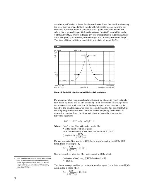
Another specification is listed for the resolution filters: bandwidth selectivity
(or selectivity or shape factor). Bandwidth selectivity helps determine the
resolving power for unequal sinusoids. For Agilent analyzers, bandwidth
selectivity is generally specified as the ratio of the 60 dB bandwidth to the
3 dB bandwidth, as shown in Figure 2-9. The analog filters in Agilent analyzers
are a four-pole, synchronously-tuned design, with a nearly Gaussian shape 4 .
This type of filter exhibits a bandwidth selectivity of about 12.7:1.
3 dB
60 dB
Figure 2-9. Bandwidth selectivity, ratio of 60 dB to 3 dB bandwidths
For example, what resolution bandwidth must we choose to resolve signals
that differ by 4 kHz and 30 dB, assuming 12.7:1 bandwidth selectivity? Since
we are concerned with rejection of the larger signal when the analyzer is
tuned to the smaller signal, we need to consider not the full bandwidth, but
the frequency difference from the filter center frequency to the skirt. To
determine how far down the filter skirt is at a given offset, we use the
following equation:
Where
H(∆f) = –10(N) log 10 [(∆f/f 0 ) 2 + 1]
H(∆f) is the filter skirt rejection in dB
N is the number of filter poles
∆f is the frequency offset from the center in Hz, and
RBW
f 0 is given by
2 √2 1/N –1
For our example, N=4 and ∆f = 4000. Let’s begin by trying the 3 kHz RBW
filter. First, we compute f 0 :
3000
f 0 =
= 3448.44
2 √2 1/4 –1
Now we can determine the filter rejection at a 4 kHz offset:
4. Some older spectrum analyzer models used five-pole
filters for the narrowest resolution bandwidths to
provide improved selectivity of about 10:1. Modern
designs achieve even better bandwidth selectivity
using digital IF filters.
18
H(4000) = –10(4) log 10 [(4000/3448.44) 2 + 1]
= –14.8 dB
This is not enough to allow us to see the smaller signal. Let’s determine H(∆f)
again using a 1 kHz filter:
1000
f 0 =
= 1149.48
2 √2 1/4 –1