Agilent Spectrum Analysis Basics - Agilent Technologies

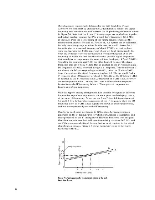
The situation is considerably different for the high band, low IF case.
As before, we shall start by plotting the LO fundamental against the signalfrequency
axis and then add and subtract the IF, producing the results shown
in Figure 7-4. Note that the 1 – and 1 + tuning ranges are much closer together,
and in fact overlap, because the IF is a much lower frequency, 321.4 MHz
in this case. Does the close spacing of the tuning ranges complicate the
measurement process? Yes and no. First of all, our system can be calibrated
for only one tuning range at a time. In this case, we would choose the 1 –
tuning to give us a low-end frequency of about 2.7 GHz, so that we have
some overlap with the 3 GHz upper end of our low band tuning range. So
what are we likely to see on the display? If we enter the graph at an LO
frequency of 5 GHz, we find that there are two possible signal frequencies
that would give us responses at the same point on the display: 4.7 and 5.3 GHz
(rounding the numbers again). On the other hand, if we enter the signal
frequency axis at 5.3 GHz, we find that in addition to the 1 + response at an
LO frequency of 5 GHz, we could also get a 1 – response. This would occur if
we allowed the LO to sweep as high as 5.6 GHz, twice the IF above 5 GHz.
Also, if we entered the signal frequency graph at 4.7 GHz, we would find a
1 + response at an LO frequency of about 4.4 GHz (twice the IF below 5 GHz)
in addition to the 1 – response at an LO frequency of 5 GHz. Thus, for every
desired response on the 1 – tuning line, there will be a second response
located twice the IF frequency below it. These pairs of responses are
known as multiple responses.
With this type of mixing arrangement, it is possible for signals at different
frequencies to produce responses at the same point on the display, that is,
at the same LO frequency. As we can see from Figure 7-4, input signals at
4.7 and 5.3 GHz both produce a response at the IF frequency when the LO
frequency is set to 5 GHz. These signals are known as image frequencies,
and are also separated by twice the IF frequency.
Clearly, we need some mechanism to differentiate between responses
generated on the 1 – tuning curve for which our analyzer is calibrated, and
those produced on the 1 + tuning curve. However, before we look at signal
identification solutions, let’s add harmonic-mixing curves to 26.5 GHz and
see if there are any additional factors that we must consider in the signal
identification process. Figure 7-5 shows tuning curves up to the fourth
harmonic of the LO.
10
Signal frequency (GHz)
5.3
4.7
Image frequencies
1+
1–
LO
0
3
4 4.4 5 5.6
LO frequency (GHz)
6
Figure 7-4. Tuning curves for fundamental mixing in the high
band, low IF case
86