Processus de Markov, de Levy, Files d'attente, Actuariat et Fiabilité ...
Processus de Markov, de Levy, Files d'attente, Actuariat et Fiabilité ...
Processus de Markov, de Levy, Files d'attente, Actuariat et Fiabilité ...

You also want an ePaper? Increase the reach of your titles
YUMPU automatically turns print PDFs into web optimized ePapers that Google loves.
L<strong>et</strong> b e (x) = ¯B(x)/m 1 = ∑ I ˜β i=1 i e −bix , where ˜β i = β i /m 1 , <strong>de</strong>note the ”stationary excess<br />
<strong>de</strong>nsity/integrated tail/lad<strong>de</strong>r distribution”, and l<strong>et</strong> b ∗ e (s) <strong>de</strong>note it’s Laplace transform.<br />
L<strong>et</strong> l(s) = κ(s) = c −λ ¯B ∗ (s), (this is the reciprocal of the Wiener-Hopf factor φ − (s)) and<br />
s<br />
l<strong>et</strong> −r i , r i > 0, i = 1, ..., I <strong>de</strong>note the non-zero (negative) roots of the ”simplified Cramér<br />
Lundberg ” equation :<br />
0 = l(s) ⇐⇒ c λ = ¯B ∗ (s) ⇐⇒ b ∗ e (s) = ρ−1 = 1 + θ ⇐⇒ c − λ<br />
I∑<br />
i=1<br />
β i<br />
1<br />
b i + s = 0<br />
Decomposing in simple fractions the Pollaczek-Khinchine formula (4.8) it follows that :<br />
( I∑<br />
)<br />
ψ ∗ (s) = 1 s − l(0)<br />
sl(s) = 1 s − C i<br />
+ 1 I∑ C i<br />
=<br />
s + r<br />
i=1 i s r<br />
i=1 i + s<br />
and therefore<br />
Therefore,<br />
ψ(x) =<br />
I∑<br />
C i e −r ix<br />
i=1<br />
ψ(x) =<br />
where C i = − κ′ (0)<br />
κ ′ (−r i )<br />
I∑<br />
C i e −r ix<br />
i=1<br />
(4.19) CLconst<br />
(4.20) Ch<br />
and thus finding the ruin probability reduces to solving the ”simplified Cramér Lundberg ”<br />
equation (??), simple fractions <strong>de</strong>composition and applying the explicit formula (4.20). Of<br />
course, the first task can only be achieved analytically in particular cases § .<br />
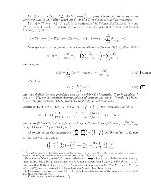
Exemple 4.7.3 L<strong>et</strong> c = 1, λ = 2, and ¯B ∗ (s) = 1 1<br />
+ 3 1<br />
. The ”simplified symbol” is :<br />
4 2+s 4 4+s<br />
( 1 1<br />
l(s) = 1 − 2<br />
4 2 + s + 3 )<br />
1 4(1 + s)(3 + s)<br />
=<br />
4 4 + s 3(s + 2)(s + 4) =⇒ r 1 = 1, r 2 = 3<br />
and the coefficients C i (obtained for example by partial fractions of ψ ∗ (s) = 1 − 3(s+2)(s+4) ,<br />
s 8s(1+s)(3+s)<br />
or by (4.19)) are : C 1 = 9/16, C 2 = 1/16.<br />
( 1<br />
) ( )<br />
1 1 −1<br />
Alternatively, the Cauchy matrix is<br />
be obtained from the system<br />
( 1 −1<br />
1<br />
3<br />
1<br />
) (C1<br />
C 2<br />
)<br />
=<br />
( 1<br />
2 1<br />
4)<br />
2−1<br />
1<br />
4−1<br />
2−3<br />
1<br />
4−3<br />
=<br />
=⇒<br />
(<br />
C1<br />
C 2<br />
)<br />
= 3 4<br />
1<br />
1<br />
3<br />
and the coefficients C i may<br />
( ) ( 1 1 1<br />
− 1 2<br />
1 1<br />
3 4)<br />
§ To g<strong>et</strong> examples of this situation, consi<strong>de</strong>r the case when b i and the roots r i are integers (for example,<br />
chose r i arbitrary un<strong>de</strong>r the necessary constraints 0 < r 1 < b 1 < r 2 ... < b I ).<br />
1<br />
Form next the ”Cauchy matrix” C A <strong>de</strong>note with elements<br />
b i−r k<br />
, i, k = 1, ..., I,, which intervenes naturally,<br />
since the Cramér Lundberg equation may also be written in system form β C A = c λ 1 where β = (β 1, ..., β I ).<br />
Note now that 1) the vector C = (C 1 , ..., C I ) satisfies the linear system C A C = b (−1) where b (−1) :=<br />
(b −1<br />
1<br />
, ..., b−1<br />
I<br />
)), and thus is compl<strong>et</strong>ely <strong>de</strong>termined once b i and r i have been chosen.<br />
2) Furthermore, we may <strong>de</strong>termine ψ(0) = ∑ i C i and the saf<strong>et</strong>y loading θ. The equation c = λm 1 (1 + θ)<br />
fixes then the quotient c/λ.<br />
3) Finally, β may be computed from (??).