Simulation numérique du mouvement et de la déformation des ...

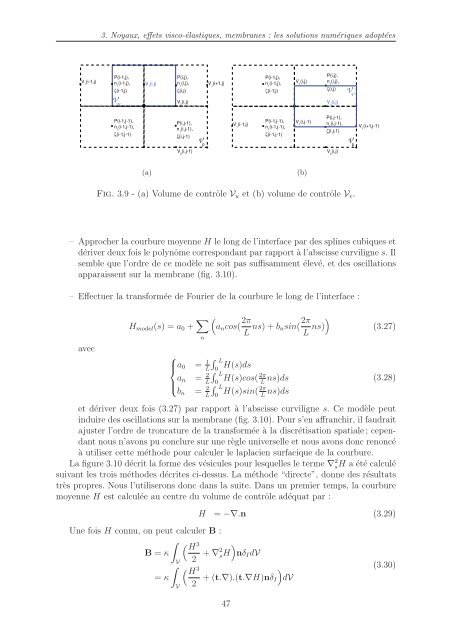
3. Noyaux, effets visco-élastiques, membranes : les solutions numériques adoptéesV 1(i-1,j)P(i-1,j),n 1(i-1,j),ζ(i-1,j)V 1(i,j)P(i,j),n 1(i,j),ζ(i,j)V 1(i+1,j)P(i-1,j),n 1(i-1,j),ζ(i-1,j)V 1(i,j)P(i,j),n 1(i,j),ζ(i,j)V VV UV 2(i,j)V 2(i,j)P(i-1,j-1),n 1(i-1,j-1),ζ(i-1,j-1)P(i,j-1),n 1(i,j-1),ζ(i,j-1)V 1(i-1,j)P(i-1,j-1),n 1(i-1,j-1),ζ(i-1,j-1)V 1(i,j-1)P(i,j-1),n 1(i,j-1),ζ(i,j-1)V 1(i+1,j-1)V pV pV 2(i,j-1)V 2(i,j)(a)(b)Fig. 3.9 - (a) Volume de contrôle V u et (b) volume de contrôle V v .– Approcher la courbure moyenne H le long de l’interface par des splines cubiques etdériver deux fois le polynôme correspondant par rapport à l’abscisse curviligne s. Ilsemble que l’ordre de ce modèle ne soit pas suffisamment élevé, et des oscillationsapparaissent sur la membrane (fig. 3.10).– Effectuer la transformée de Fourier de la courbure le long de l’interface :H model (s) =a 0 + ∑ n(a n cos( 2π L ns)+b nsin( 2π L ns) )(3.27)avec⎧⎪⎨⎪⎩a 0a nb n= 1 L= 2 L= 2 L∫ L H(s)ds∫0L H(s)cos( 2πns)ds(3.28)∫0L LH(s)sin( 2πns)ds L0et dériver deux fois (3.27) par rapport à l’abscisse curviligne s. Cemodèle peutinduire des oscillations sur la membrane (fig. 3.10). Pour s’en affranchir, il faudraitajuster l’ordre de troncature de la transformée à la discrétisation spatiale ; cependantnous n’avons pu conclure sur une règle universelle et nous avons donc renoncéà utiliser cette méthode pour calculer le laplacien surfacique de la courbure.La figure 3.10 décrit la forme des vésicules pour lesquelles le terme ∇ 2 sH aété calculésuivant les trois méthodes décrites ci-dessus. La méthode “directe”, donne des résultatstrès propres. Nous l’utiliserons donc dans la suite. Dans un premier temps, la courburemoyenne H est calculée au centre du volume de contrôle adéquat par :Une fois H connu, on peut calculer B :∫ ( H3 )B = κV 2 + ∇2 sH nδ I dV∫ ( H3)= κ2 +(t.∇).(t.∇H)nδ I dVVH = −∇.n (3.29)47(3.30)