AnÃ¡lise do Efeito do Risco de Cheia no Valor de ImÃ³veis pelo ...

More documents

Recommendations

Info

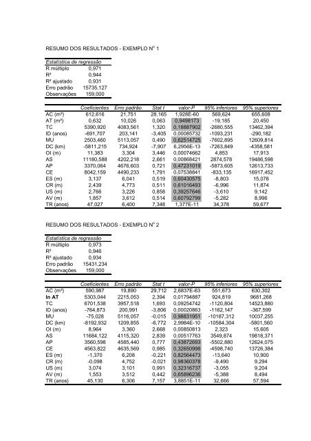
RESUMO DOS RESULTADOS - EXEMPLO N o 1 Estatística de regressão R múltiplo 0,971 R² 0,944 R² ajustado 0,931 Erro padrão 15735,127 Observações 159,000 Coeficientes Erro padrão Stat t valor-P 95% inferiores 95% superiores AC (m²) 612,616 21,751 28,165 1,928E-60 569,624 655,608 AT (m²) 0,632 10,026 0,063 0,9498173 -19,185 20,450 TC 5390,920 4083,561 1,320 0,18887902 -2680,555 13462,394 ID (anos) -691,707 203,141 -3,405 0,00085732 -1093,231 -290,182 MUM 2503,460 5113,057 0,490 0,62514725 -7602,895 12609,814 DC (km) -5811,215 734,924 -7,907 6,2956E-13 -7263,849 -4358,581 OI (m) 11,383 3,304 3,446 0,00074662 4,853 17,913 AS 11180,588 4202,218 2,661 0,00868421 2874,578 19486,598 AP 3370,064 4676,603 0,721 0,47231019 -5873,605 12613,733 CE 8042,159 4490,233 1,791 0,07538841 -833,135 16917,452 ES (m) 3,137 6,041 0,519 0,60430575 -8,803 15,078 CR (m) 2,439 4,773 0,511 0,61016493 -6,996 11,874 US (m) 2,766 3,226 0,858 0,39257646 -3,610 9,142 AV (m) 1,857 3,612 0,514 0,60792799 -5,282 8,996 TR (anos) 47,027 6,400 7,348 1,377E-11 34,378 59,677 RESUMO DOS RESULTADOS - EXEMPLO N o 2 Estatística de regressão R múltiplo 0,973 R² 0,946 R² ajustado 0,934 Erro padrão 15431,234 Observações 159,000 Coeficientes Erro padrão Stat t valor-P 95% inferiores 95% superiores AC (m²) 590,987 19,890 29,712 2,6837E-63 551,673 630,302 ln AT 5303,044 2215,053 2,394 0,01794887 924,819 9681,268 TC 6701,538 3957,518 1,693 0,09254742 -1120,804 14523,880 ID (anos) -764,873 200,991 -3,806 0,00020863 -1162,147 -367,599 MUM -75,028 5116,057 -0,015 0,98831951 -10187,312 10037,255 DC (km) -8192,932 1209,855 -6,772 2,9984E-10 -10584,304 -5801,560 OI (m) 8,964 3,360 2,668 0,00850813 2,323 15,605 AS 11684,122 4115,320 2,839 0,00517763 3549,874 19818,371 AP 3560,598 4585,440 0,777 0,43872693 -5502,880 12624,075 CE 4563,822 4635,569 0,985 0,32650998 -4598,740 13726,384 ES (m) -1,370 6,208 -0,221 0,82564473 -13,640 10,900 CR (m) -0,098 4,752 -0,021 0,98360378 -9,490 9,294 US (m) 3,074 3,101 0,991 0,32316737 -3,055 9,204 AV (m) 1,553 3,512 0,442 0,65896236 -5,388 8,494 TR (anos) 45,130 6,306 7,157 3,8851E-11 32,666 57,594
RESUMO DOS RESULTADOS - EXEMPLO N o 3 Estatística de regressão R múltiplo 0,972 R² 0,944 R² ajustado 0,932 Erro padrão 15649,110 Observações 159,000 Coeficientes Erro padrão Stat t valor-P 95% inferiores 95% superiores AC (m²) 581,774 20,781 27,996 4,0208E-60 540,699 622,848 ln AT 9539,677 2901,263 3,288 0,0012676 3805,105 15274,249 TC 7147,705 4045,019 1,767 0,07934017 -847,589 15142,999 ID (anos) -805,339 203,658 -3,954 0,00011992 -1207,884 -402,794 MUM 4061,488 5099,257 0,796 0,42706058 -6017,588 14140,565 ln DC -45518,744 7143,075 -6,372 2,3601E-09 -59637,585 -31399,903 OI (m) 8,875 3,451 2,572 0,01112159 2,055 15,695 AS 11547,932 4179,339 2,763 0,00647349 3287,145 19808,720 AP 3947,723 4670,324 0,845 0,3993579 -5283,535 13178,981 CE 8259,981 4564,774 1,810 0,07245827 -762,650 17282,611 ES (m) 1,006 6,256 0,161 0,87241915 -11,360 13,373 CR (m) 1,588 4,794 0,331 0,74092779 -7,887 11,063 US (m) 3,162 3,149 1,004 0,31693109 -3,062 9,386 AV (m) -1,069 3,464 -0,309 0,75806945 -7,916 5,778 TR (anos) 43,464 6,389 6,803 2,5412E-10 30,836 56,091 RESUMO DOS RESULTADOS - EXEMPLO N o 4 Estatística de regressão R múltiplo 0,973 R² 0,947 R² ajustado 0,935 Erro padrão 15245,469 Observações 159,000 Coeficientes Erro padrão Stat t valor-P 95% inferiores 95% superiores AC (m²) 592,751 19,668 30,137 4,6046E-64 553,875 631,627 ln AT 3335,801 2235,092 1,492 0,13776446 -1082,032 7753,635 TC 4841,877 3966,907 1,221 0,22424477 -2999,022 12682,776 ID (anos) -825,890 198,282 -4,165 5,3361E-05 -1217,809 -433,970 MUM 124,129 5052,946 0,025 0,98043542 -9863,411 10111,669 DC (km) -8581,630 1198,639 -7,159 3,8254E-11 -10950,833 -6212,426 OI (m) 9,314 3,298 2,824 0,00541464 2,795 15,833 AS 11958,973 4064,617 2,942 0,00379914 3924,943 19993,004 AP 2454,453 4523,705 0,543 0,58826072 -6487,002 11395,907 CE 3037,956 4555,591 0,667 0,50592667 -5966,523 12042,435 ES (m) -2,854 6,093 -0,468 0,64016418 -14,897 9,189 CR (m) 1,327 4,695 0,283 0,77782537 -7,953 10,607 US (m) 3,222 3,064 1,052 0,29478785 -2,834 9,277 AV (m) 2,038 3,473 0,587 0,55818795 -4,826 8,903 ln TR 6334,705 846,486 7,484 6,5841E-12 4661,560 8007,850
Page 1 and 2:
LIZANDRA MARTINEZ LEZCANO ANÁLISE
Page 3 and 4:
Aos meus queridos pais, pelo consta
Page 5 and 6:
SUMÁRIO LISTA DE TABELAS..........
Page 7 and 8:
5.2.3.3 Avaliação do atributo amb
Page 9 and 10:
LISTA DE FIGURAS FIGURA 2.1 - EVOLU
Page 11 and 12:
MU OI OLS P PIB RMC SANEPAR SIGRH S
Page 13 and 14:
ABSTRACT This work proposes a metho
Page 15 and 16:
2 estadual, acabou atraindo uma gra
Page 17 and 18:
4 de se avaliar a eficiência econ
Page 19 and 20:
6 2 A PROBLEMÁTICA DAS INUNDAÇÕE
Page 21 and 22:
8 econômico. Os efeitos desse proc
Page 23 and 24:
10 Além das colocações citadas,
Page 25 and 26:
12 direta e indiretamente, por um g
Page 27 and 28:
14 Curitiba e alguns municípios da
Page 29 and 30:
16 seus habitantes. De acordo com T
Page 31 and 32:
18 De acordo com OSTROWSKY (2000),
Page 33 and 34:
20 liberação defasada, e com pico
Page 35 and 36:
22 podendo ser um meio efetivo de c
Page 37 and 38:
24 de pertences (móveis e utensíl
Page 39 and 40:
26 projetos relacionados com recurs
Page 41 and 42:
28 privado, a análise é feita pro
Page 43 and 44:
30 prejuízos da interrupção de a
Page 45 and 46:
32 (ACB), que pode ser feita com ba
Page 47 and 48:
34 Finalmente, cabe mencionar que,
Page 49 and 50:
36 intervenções de drenagem urban
Page 51 and 52:
38 Entretanto, cabe mencionar que,
Page 53 and 54:
40 que ainda não estão sedimentad
Page 55 and 56:
42 A bacia hidrográfica, com toda
Page 57 and 58:
44 prejuízos para a sociedade. Na
Page 59 and 60:
46 3 VALORAÇÃO ECONÔMICA DO MEIO
Page 61 and 62:
48 afirmar que a valoração monet
Page 63 and 64:
50 complexas relações da biodiver
Page 65 and 66:
52 não. Quando não é possível o
Page 67 and 68:
54 uso indireto (VUI) e valor de op
Page 69 and 70:
56 opção ou de existência. Assim
Page 71 and 72:
58 Bateman & Turner (1992, p.123) p
Page 73 and 74:
60 produto, é possível estimar in
Page 75 and 76:
62 Com relação à aplicabilidade
Page 77 and 78:
64 os custos incorridos na reposiç
Page 79 and 80:
66 (iv) Custos de oportunidade: Seg
Page 81 and 82:
68 deste bem, obter um indicador do
Page 83 and 84:
70 Vi = f(CVi ,S1,S 2 ,...,S n ) (3
Page 85 and 86:
72 consumidor em situações hipote
Page 87 and 88:
74 TABELA 3.1 - COMPARAÇÃO ENTRE
Page 89 and 90:
76 4 MÉTODO DOS PREÇOS HEDÔNICOS
Page 91 and 92:
78 método dos preços hedônicos.
Page 93 and 94:
80 No âmbito da valoração ambien
Page 95 and 96:
82 normal de média nula, (2) as va
Page 97 and 98:
84 características que possam infl
Page 99 and 100:
86 4.3 REGRESSÃO LINEAR MÚLTIPLA
Page 101 and 102:
88 • O vetor dos erros ε é alea
Page 103 and 104:
90 pela seguinte expressão: −1 b
Page 105 and 106:
92 onde 1 é um vetor de elementos
Page 107 and 108:
94 T β ∗ = i i (4.27) s − β a
Page 109 and 110:
96 nula implica em não poder consi
Page 111 and 112:
98 diferenciais nos preços de prop
Page 113 and 114:
100 TABELA 4.1 - ESTUDOS RELATIVOS
Page 115 and 116:
102 Belo Horizonte, salientando que
Page 117 and 118:
104 foi utilizado o método dos pre
Page 119 and 120:
106 coleta de dados detalhada e cui
Page 121 and 122:
108 5 ESTUDO DE CASO 5.1 CARACTERIZ
Page 123 and 124:
110 Com relação à ocupação do
Page 125 and 126:
112 benefícios quantificados atrav
Page 127 and 128:
114 variáveis definidas para serem
Page 129 and 130:
116 Nesta etapa foi realizado um gr
Page 131 and 132:
118 5.2.2 Levantamento dos Valores
Page 133 and 134:
120 e 25 anos de retorno. TABELA 5.
Page 135 and 136:
122 5.2.3 Avaliação dos Atributos
Page 137 and 138: 124 Esta variável, portanto, para
Page 139 and 140: 126 qualidade do pavimento disponib
Page 141 and 142: 128 considerar este atributo na an
Page 143 and 144: 130 grandes cidades, passando a exe
Page 145 and 146: 132 Vale a pena relembrar que o per
Page 147 and 148: 134 Finalmente, para cada um destes
Page 149 and 150: 136 5.2.5 Formulação do Modelo Ma
Page 151 and 152: 138 utilizados. Uma vez definido o
Page 153 and 154: 140 A escolha dos atributos para o
Page 155 and 156: 142 TABELA 5.2 - DESCRIÇÃO DAS VA
Page 157 and 158: 144 quantitativa da variável, ou s
Page 159 and 160: 146 AV = proximidade a áreas verde
Page 161 and 162: 148 localizado em Curitiba influenc
Page 163 and 164: 150 O número de graus de liberdade
Page 165 and 166: 152 Neste caso, resultaria convenie
Page 167 and 168: 154 anti-pó como tipo de pavimento
Page 169 and 170: 156 FIGURA 5.4 - AVALIAÇÃO DE BEN
Page 171 and 172: 158 Finalmente deve-se considerar q
Page 173 and 174: 160 onde se dispõe de dados; (v) O
Page 175 and 176: 162 REFERÊNCIAS BAPTISTA, M. B.; N
Page 177 and 178: 164 LOUCKS, D. P.; STEDINGER, J. R.
Page 179 and 180: 166 TAVARES, V. E.; LANNA, A. E. A
Page 181 and 182: Tabela A1 - Informações coletadas
Page 187: ANEXO C - EXEMPLOS DE REGRESSÕES T
Page 191 and 192: RESUMO DOS RESULTADOS - EXEMPLO N o
Page 197: RESUMO DOS RESULTADOS - EXEMPLO N o
show all

AnÃ¡lise do Efeito do Risco de Cheia no Valor de ImÃ³veis pelo ...

You also want an ePaper? Increase the reach of your titles

Delete template?

Save as template?