AnÃ¡lise do Efeito do Risco de Cheia no Valor de ImÃ³veis pelo ...

More documents

Recommendations

Info

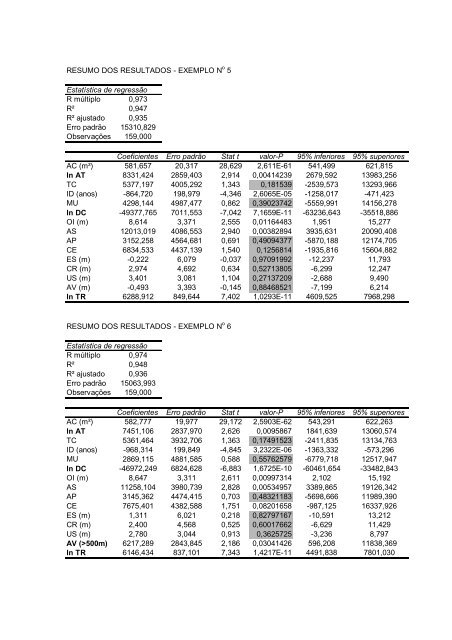
RESUMO DOS RESULTADOS - EXEMPLO N o 5 Estatística de regressão R múltiplo 0,973 R² 0,947 R² ajustado 0,935 Erro padrão 15310,829 Observações 159,000 Coeficientes Erro padrão Stat t valor-P 95% inferiores 95% superiores AC (m²) 581,657 20,317 28,629 2,611E-61 541,499 621,815 ln AT 8331,424 2859,403 2,914 0,00414239 2679,592 13983,256 TC 5377,197 4005,292 1,343 0,181539 -2539,573 13293,966 ID (anos) -864,720 198,979 -4,346 2,6065E-05 -1258,017 -471,423 MUM 4298,144 4987,477 0,862 0,39023742 -5559,991 14156,278 ln DC -49377,765 7011,553 -7,042 7,1659E-11 -63236,643 -35518,886 OI (m) 8,614 3,371 2,555 0,01164483 1,951 15,277 AS 12013,019 4086,553 2,940 0,00382894 3935,631 20090,408 AP 3152,258 4564,681 0,691 0,49094377 -5870,188 12174,705 CE 6834,533 4437,139 1,540 0,1256814 -1935,816 15604,882 ES (m) -0,222 6,079 -0,037 0,97091992 -12,237 11,793 CR (m) 2,974 4,692 0,634 0,52713805 -6,299 12,247 US (m) 3,401 3,081 1,104 0,27137209 -2,688 9,490 AV (m) -0,493 3,393 -0,145 0,88468521 -7,199 6,214 ln TR 6288,912 849,644 7,402 1,0293E-11 4609,525 7968,298 RESUMO DOS RESULTADOS - EXEMPLO N o 6 Estatística de regressão R múltiplo 0,974 R² 0,948 R² ajustado 0,936 Erro padrão 15063,993 Observações 159,000 Coeficientes Erro padrão Stat t valor-P 95% inferiores 95% superiores AC (m²) 582,777 19,977 29,172 2,5903E-62 543,291 622,263 ln AT 7451,106 2837,970 2,626 0,0095867 1841,639 13060,574 TC 5361,464 3932,706 1,363 0,17491523 -2411,835 13134,763 ID (anos) -968,314 199,849 -4,845 3,2322E-06 -1363,332 -573,296 MUM 2869,115 4881,585 0,588 0,55762579 -6779,718 12517,947 ln DC -46972,249 6824,628 -6,883 1,6725E-10 -60461,654 -33482,843 OI (m) 8,647 3,311 2,611 0,00997314 2,102 15,192 AS 11258,104 3980,739 2,828 0,00534957 3389,865 19126,342 AP 3145,362 4474,415 0,703 0,48321183 -5698,666 11989,390 CE 7675,401 4382,588 1,751 0,08201658 -987,125 16337,926 ES (m) 1,311 6,021 0,218 0,82797167 -10,591 13,212 CR (m) 2,400 4,568 0,525 0,60017662 -6,629 11,429 US (m) 2,780 3,044 0,913 0,3625725 -3,236 8,797 AV (>500m) 6217,289 2843,845 2,186 0,03041426 596,208 11838,369 ln TR 6146,434 837,101 7,343 1,4217E-11 4491,838 7801,030
RESUMO DOS RESULTADOS - EXEMPLO N o 7 Estatística de regressão R múltiplo 0,974 R² 0,949 R² ajustado 0,937 Erro padrão 15014,813 Observações 159,000 Coeficientes Erro padrão Stat t valor-P 95% inferiores 95% superiores AC (m²) 578,679 19,738 29,318 1,3989E-62 539,666 617,692 ln AT 8627,615 2708,853 3,185 0,00177489 3273,357 13981,873 TC 6882,875 3880,909 1,774 0,07825611 -788,043 14553,794 ID (anos) -940,903 199,584 -4,714 5,668E-06 -1335,397 -546,409 MUM 3223,273 4841,042 0,666 0,5065899 -6345,421 12791,968 ln DC -46783,653 6794,998 -6,885 1,6527E-10 -60214,495 -33352,812 OI (m) 8,479 3,282 2,583 0,01077671 1,992 14,966 AS 11264,088 3961,638 2,843 0,00511483 3433,604 19094,572 AP 3183,143 4457,591 0,714 0,47632443 -5627,632 11993,917 CE 6905,685 4356,226 1,585 0,1151043 -1704,733 15516,104 ES (>500m) -3416,468 2625,204 -1,301 0,19519622 -8605,387 1772,451 CR (>500m) -1634,676 2683,815 -0,609 0,54342667 -6939,444 3670,092 US (>500m) -3292,274 2749,362 -1,197 0,23309142 -8726,601 2142,052 AV (>500m) 6033,535 2836,249 2,127 0,03509959 427,470 11639,601 ln TR 5986,858 828,138 7,229 2,6257E-11 4349,980 7623,737 RESUMO DOS RESULTADOS - EXEMPLO N o 8 Estatística de regressão R múltiplo 0,974 R² 0,949 R² ajustado 0,937 Erro padrão 14982,210 Observações 159,000 Coeficientes Erro padrão Stat t valor-P 95% inferiores 95% superiores AC (m²) 579,935 19,587 29,608 2,3892E-63 541,222 618,648 ln AT 8636,289 2702,933 3,195 0,00171513 3294,051 13978,527 TC 6919,983 3872,005 1,787 0,07599686 -732,877 14572,844 ID (anos) -918,161 195,635 -4,693 6,1661E-06 -1304,825 -531,497 MUM 2802,585 4781,113 0,586 0,55866705 -6647,090 12252,260 ln DC -47326,500 6721,669 -7,041 7,0744E-11 -60611,605 -34041,395 OI (m) 8,623 3,266 2,640 0,00919425 2,168 15,079 AS 11363,110 3949,705 2,877 0,00462211 3556,678 19169,542 AP 3334,743 4440,973 0,751 0,45392752 -5442,659 12112,145 CE 6627,736 4322,851 1,533 0,12740897 -1916,204 15171,676 ES (>500m) -3151,763 2583,360 -1,220 0,22443603 -8257,668 1954,142 US (>500m) -3440,345 2732,646 -1,259 0,21006097 -8841,309 1960,620 AV (>500m) 6018,904 2829,989 2,127 0,03512703 425,547 11612,262 ln TR 5988,659 826,334 7,247 2,3295E-11 4355,443 7621,875
Page 1 and 2:
LIZANDRA MARTINEZ LEZCANO ANÁLISE
Page 3 and 4:
Aos meus queridos pais, pelo consta
Page 5 and 6:
SUMÁRIO LISTA DE TABELAS..........
Page 7 and 8:
5.2.3.3 Avaliação do atributo amb
Page 9 and 10:
LISTA DE FIGURAS FIGURA 2.1 - EVOLU
Page 11 and 12:
MU OI OLS P PIB RMC SANEPAR SIGRH S
Page 13 and 14:
ABSTRACT This work proposes a metho
Page 15 and 16:
2 estadual, acabou atraindo uma gra
Page 17 and 18:
4 de se avaliar a eficiência econ
Page 19 and 20:
6 2 A PROBLEMÁTICA DAS INUNDAÇÕE
Page 21 and 22:
8 econômico. Os efeitos desse proc
Page 23 and 24:
10 Além das colocações citadas,
Page 25 and 26:
12 direta e indiretamente, por um g
Page 27 and 28:
14 Curitiba e alguns municípios da
Page 29 and 30:
16 seus habitantes. De acordo com T
Page 31 and 32:
18 De acordo com OSTROWSKY (2000),
Page 33 and 34:
20 liberação defasada, e com pico
Page 35 and 36:
22 podendo ser um meio efetivo de c
Page 37 and 38:
24 de pertences (móveis e utensíl
Page 39 and 40:
26 projetos relacionados com recurs
Page 41 and 42:
28 privado, a análise é feita pro
Page 43 and 44:
30 prejuízos da interrupção de a
Page 45 and 46:
32 (ACB), que pode ser feita com ba
Page 47 and 48:
34 Finalmente, cabe mencionar que,
Page 49 and 50:
36 intervenções de drenagem urban
Page 51 and 52:
38 Entretanto, cabe mencionar que,
Page 53 and 54:
40 que ainda não estão sedimentad
Page 55 and 56:
42 A bacia hidrográfica, com toda
Page 57 and 58:
44 prejuízos para a sociedade. Na
Page 59 and 60:
46 3 VALORAÇÃO ECONÔMICA DO MEIO
Page 61 and 62:
48 afirmar que a valoração monet
Page 63 and 64:
50 complexas relações da biodiver
Page 65 and 66:
52 não. Quando não é possível o
Page 67 and 68:
54 uso indireto (VUI) e valor de op
Page 69 and 70:
56 opção ou de existência. Assim
Page 71 and 72:
58 Bateman & Turner (1992, p.123) p
Page 73 and 74:
60 produto, é possível estimar in
Page 75 and 76:
62 Com relação à aplicabilidade
Page 77 and 78:
64 os custos incorridos na reposiç
Page 79 and 80:
66 (iv) Custos de oportunidade: Seg
Page 81 and 82:
68 deste bem, obter um indicador do
Page 83 and 84:
70 Vi = f(CVi ,S1,S 2 ,...,S n ) (3
Page 85 and 86:
72 consumidor em situações hipote
Page 87 and 88:
74 TABELA 3.1 - COMPARAÇÃO ENTRE
Page 89 and 90:
76 4 MÉTODO DOS PREÇOS HEDÔNICOS
Page 91 and 92:
78 método dos preços hedônicos.
Page 93 and 94:
80 No âmbito da valoração ambien
Page 95 and 96:
82 normal de média nula, (2) as va
Page 97 and 98:
84 características que possam infl
Page 99 and 100:
86 4.3 REGRESSÃO LINEAR MÚLTIPLA
Page 101 and 102:
88 • O vetor dos erros ε é alea
Page 103 and 104:
90 pela seguinte expressão: −1 b
Page 105 and 106:
92 onde 1 é um vetor de elementos
Page 107 and 108:
94 T β ∗ = i i (4.27) s − β a
Page 109 and 110:
96 nula implica em não poder consi
Page 111 and 112:
98 diferenciais nos preços de prop
Page 113 and 114:
100 TABELA 4.1 - ESTUDOS RELATIVOS
Page 115 and 116:
102 Belo Horizonte, salientando que
Page 117 and 118:
104 foi utilizado o método dos pre
Page 119 and 120:
106 coleta de dados detalhada e cui
Page 121 and 122:
108 5 ESTUDO DE CASO 5.1 CARACTERIZ
Page 123 and 124:
110 Com relação à ocupação do
Page 125 and 126:
112 benefícios quantificados atrav
Page 127 and 128:
114 variáveis definidas para serem
Page 129 and 130:
116 Nesta etapa foi realizado um gr
Page 131 and 132:
118 5.2.2 Levantamento dos Valores
Page 133 and 134:
120 e 25 anos de retorno. TABELA 5.
Page 135 and 136:
122 5.2.3 Avaliação dos Atributos
Page 137 and 138:
124 Esta variável, portanto, para
Page 139 and 140: 126 qualidade do pavimento disponib
Page 141 and 142: 128 considerar este atributo na an
Page 143 and 144: 130 grandes cidades, passando a exe
Page 145 and 146: 132 Vale a pena relembrar que o per
Page 147 and 148: 134 Finalmente, para cada um destes
Page 149 and 150: 136 5.2.5 Formulação do Modelo Ma
Page 151 and 152: 138 utilizados. Uma vez definido o
Page 153 and 154: 140 A escolha dos atributos para o
Page 155 and 156: 142 TABELA 5.2 - DESCRIÇÃO DAS VA
Page 157 and 158: 144 quantitativa da variável, ou s
Page 159 and 160: 146 AV = proximidade a áreas verde
Page 161 and 162: 148 localizado em Curitiba influenc
Page 163 and 164: 150 O número de graus de liberdade
Page 165 and 166: 152 Neste caso, resultaria convenie
Page 167 and 168: 154 anti-pó como tipo de pavimento
Page 169 and 170: 156 FIGURA 5.4 - AVALIAÇÃO DE BEN
Page 171 and 172: 158 Finalmente deve-se considerar q
Page 173 and 174: 160 onde se dispõe de dados; (v) O
Page 175 and 176: 162 REFERÊNCIAS BAPTISTA, M. B.; N
Page 177 and 178: 164 LOUCKS, D. P.; STEDINGER, J. R.
Page 179 and 180: 166 TAVARES, V. E.; LANNA, A. E. A
Page 181 and 182: Tabela A1 - Informações coletadas
Page 187 and 188: ANEXO C - EXEMPLOS DE REGRESSÕES T
Page 189: RESUMO DOS RESULTADOS - EXEMPLO N o
Page 193 and 194: RESUMO DOS RESULTADOS - EXEMPLO N o
Page 195 and 196: RESUMO DOS RESULTADOS - EXEMPLO N o
Page 197: RESUMO DOS RESULTADOS - EXEMPLO N o
show all

AnÃ¡lise do Efeito do Risco de Cheia no Valor de ImÃ³veis pelo ...

Create successful ePaper yourself

Delete template?

Save as template?