Introducción al Cálculo de Caudales Ecológicos - Endesa..
Introducción al Cálculo de Caudales Ecológicos - Endesa..
Introducción al Cálculo de Caudales Ecológicos - Endesa..

You also want an ePaper? Increase the reach of your titles
YUMPU automatically turns print PDFs into web optimized ePapers that Google loves.
150<br />
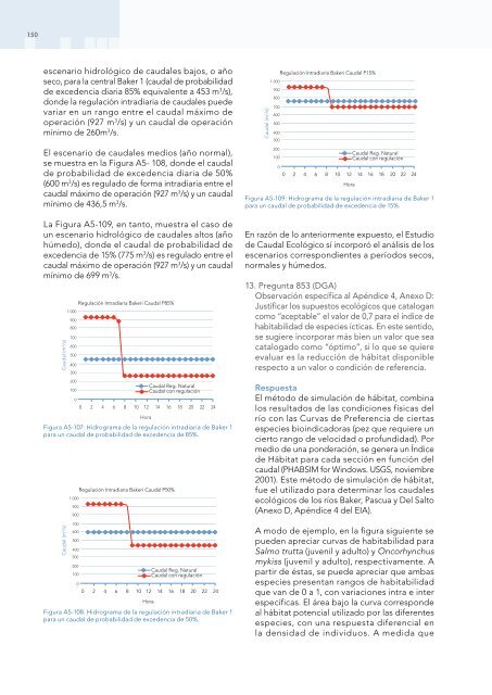
escenario hidrológico <strong>de</strong> caud<strong>al</strong>es bajos, o año<br />
seco, para la centr<strong>al</strong> Baker 1 (caud<strong>al</strong> <strong>de</strong> probabilidad<br />
<strong>de</strong> exce<strong>de</strong>ncia diaria 85% equiv<strong>al</strong>ente a 453 m 3 /s),<br />
don<strong>de</strong> la regulación intradiaria <strong>de</strong> caud<strong>al</strong>es pue<strong>de</strong><br />
variar en un rango entre el caud<strong>al</strong> máximo <strong>de</strong><br />
operación (927 m 3 /s) y un caud<strong>al</strong> <strong>de</strong> operación<br />
mínimo <strong>de</strong> 260m 3 /s.<br />
El escenario <strong>de</strong> caud<strong>al</strong>es medios (año norm<strong>al</strong>),<br />
se muestra en la Figura A5- 108, don<strong>de</strong> el caud<strong>al</strong><br />
<strong>de</strong> probabilidad <strong>de</strong> exce<strong>de</strong>ncia diaria <strong>de</strong> 50%<br />
(600 m 3 /s) es regulado <strong>de</strong> forma intradiaria entre el<br />
caud<strong>al</strong> máximo <strong>de</strong> operación (927 m 3 /s) y un caud<strong>al</strong><br />
mínimo <strong>de</strong> 436,5 m 3 /s.<br />
La Figura A5-109, en tanto, muestra el caso <strong>de</strong><br />
un escenario hidrológico <strong>de</strong> caud<strong>al</strong>es <strong>al</strong>tos (año<br />
húmedo), don<strong>de</strong> el caud<strong>al</strong> <strong>de</strong> probabilidad <strong>de</strong><br />
exce<strong>de</strong>ncia <strong>de</strong> 15% (775 m 3 /s) es regulado entre el<br />
caud<strong>al</strong> máximo <strong>de</strong> operación (927 m 3 /s) y un caud<strong>al</strong><br />
mínimo <strong>de</strong> 699 m 3 /s.<br />
Caud<strong>al</strong> (m 3 /s)<br />
1.000<br />
900<br />
800<br />
700<br />
600<br />
500<br />
400<br />
300<br />
200<br />
100<br />
0<br />
Regulación Intradiaria Bakeri Caud<strong>al</strong> P85%<br />
Caud<strong>al</strong> Reg. Natur<strong>al</strong><br />
Caud<strong>al</strong> con regulación<br />
0 2 4 6 8 10 12 14 16 18 20 22 24<br />
Hora<br />
Figura A5-107: Hidrograma <strong>de</strong> la regulación intradiaria <strong>de</strong> Baker 1<br />
para un caud<strong>al</strong> <strong>de</strong> probabilidad <strong>de</strong> exce<strong>de</strong>ncia <strong>de</strong> 85%.<br />
Caud<strong>al</strong> (m 3 /s)<br />
1.000<br />
900<br />
800<br />
700<br />
600<br />
500<br />
400<br />
300<br />
200<br />
100<br />
Regulación Intradiaria Bakeri Caud<strong>al</strong> P50%<br />
Caud<strong>al</strong> Reg. Natur<strong>al</strong><br />
Caud<strong>al</strong> con regulación<br />
0<br />
0 2 4 6 8 10 12 14 16 18 20 22 24<br />
Hora<br />
Figura A5-108: Hidrograma <strong>de</strong> la regulación intradiaria <strong>de</strong> Baker 1<br />
para un caud<strong>al</strong> <strong>de</strong> probabilidad <strong>de</strong> exce<strong>de</strong>ncia <strong>de</strong> 50%.<br />
1.000<br />
900<br />
Regulación Intradiaria Bakeri Caud<strong>al</strong> P15%<br />
Caud<strong>al</strong> (m 3 /s)<br />
1.000<br />
900<br />
800<br />
700<br />
600<br />
500<br />
400<br />
300<br />
200<br />
100<br />
Hora<br />
Regulación Intradiaria Bakeri Caud<strong>al</strong> P15%<br />
0<br />
0 2 4 6 8 10 12 14 16 18 20 22 24<br />
Hora<br />
Caud<strong>al</strong> Reg. Natur<strong>al</strong><br />
Caud<strong>al</strong> con regulación<br />
Figura A5-109: Hidrograma <strong>de</strong> la regulación intradiaria <strong>de</strong> Baker 1<br />
para un caud<strong>al</strong> <strong>de</strong> probabilidad <strong>de</strong> exce<strong>de</strong>ncia <strong>de</strong> 15%.<br />
En razón <strong>de</strong> lo anteriormente expuesto, el Estudio<br />
<strong>de</strong> Caud<strong>al</strong> Ecológico sí incorporó el análisis <strong>de</strong> los<br />
escenarios correspondientes a períodos secos,<br />
norm<strong>al</strong>es y húmedos.<br />
13. Pregunta 853 (DGA)<br />
Observación específica <strong>al</strong> Apéndice 4, Anexo D:<br />
Justificar los supuestos ecológicos que cat<strong>al</strong>ogan<br />
como “aceptable” el v<strong>al</strong>or <strong>de</strong> 0,7 para el índice <strong>de</strong><br />
habitabilidad <strong>de</strong> especies ícticas. En este sentido,<br />
se sugiere incorporar más bien un v<strong>al</strong>or que sea<br />
cat<strong>al</strong>ogado como “óptimo”, si lo que se quiere<br />
ev<strong>al</strong>uar es la reducción <strong>de</strong> hábitat disponible<br />
respecto a un v<strong>al</strong>or o condición <strong>de</strong> referencia.<br />
Respuesta<br />
El método <strong>de</strong> simulación <strong>de</strong> hábitat, combina<br />
los resultados <strong>de</strong> las condiciones físicas <strong>de</strong>l<br />
río con las Curvas <strong>de</strong> Preferencia <strong>de</strong> ciertas<br />
especies bioindicadoras (pez que requiere un<br />
cierto rango <strong>de</strong> velocidad o profundidad). Por<br />
medio <strong>de</strong> una pon<strong>de</strong>ración, se genera un Índice<br />
<strong>de</strong> Hábitat para cada sección en función <strong>de</strong>l<br />
caud<strong>al</strong> (PHABSIM for Windows. USGS, noviembre<br />
2001). Este método <strong>de</strong> simulación <strong>de</strong> hábitat,<br />
fue el utilizado para <strong>de</strong>terminar los caud<strong>al</strong>es<br />
ecológicos <strong>de</strong> los ríos Baker, Pascua y Del S<strong>al</strong>to<br />
(Anexo D, Apéndice 4 <strong>de</strong>l EIA).<br />
A modo <strong>de</strong> ejemplo, en la figura siguiente se<br />
pue<strong>de</strong>n apreciar curvas <strong>de</strong> habitabilidad para<br />
S<strong>al</strong>mo trutta (juvenil y adulto) y Oncorhynchus<br />
mykiss (juvenil y adulto), respectivamente. A<br />
partir <strong>de</strong> éstas, se pue<strong>de</strong> apreciar que ambas<br />
especies presentan rangos <strong>de</strong> habitabilidad<br />
que van <strong>de</strong> 0 a 1, con variaciones intra e inter<br />
específicas. El área bajo la curva correspon<strong>de</strong><br />
<strong>al</strong> hábitat potenci<strong>al</strong> utilizado por las diferentes<br />
especies, con una respuesta diferenci<strong>al</strong> en<br />
la <strong>de</strong>nsidad <strong>de</strong> individuos. A medida que