Airborne Gravity 2010 - Geoscience Australia

Airborne Gravity 2010
DEM resolution in terrain correction
Airborne gravity gradiometry data are invariably low-pass filtered versions of the actual gradient fields
because of the use of low-pass filters in the acquisition system and post-acquisition processing. The
filtering is predominantly applied in the direction of the flight lines. The exact properties of the filters
are often proprietary to the acquisition companies (Lane, 2004), and the exact parameters may not be
supplied to the end user. Regardless, the effect of filtering of the data on the resolution requirements
for terrain correction needs to be examined.
We examine this aspect by processing a set of high resolution LiDAR data at different effective
resolutions, both with and without a representative acquisition filter applied to the forward model Tzz
component of the gravity gradient (Figure 4a).
By comparing ground gravity data and airborne gravity gradient data, Lane (2004) showed that the
remaining frequency content of gravity gradiometry data after filtering may be modelled by a simple
Butterworth filter of varying cutoff wavenumber. For many currently available datasets, this filter cutoff
is approximately 200 m. Although this does not specify the actual parameters that were used for the
acquisition low-pass filter, it does provide a composite filter representation that encapsulates the
cumulative filtering effect of the acquisition system and subsequent processing steps. We therefore
used a 200 m length, fourth-order Butterworth filter applied along the “flight” direction (east-west) to
simulate the acquisition filter (Figure 4b).
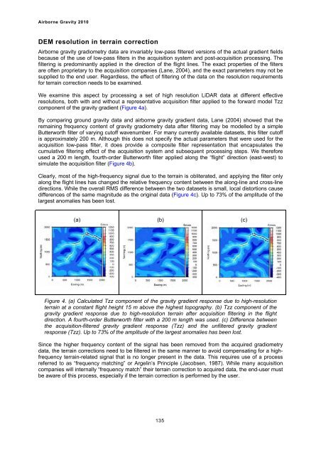
Clearly, most of the high-frequency signal due to the terrain is obliterated, and applying the filter only
along the flight lines has changed the relative frequency content between the along-line and cross-line
directions. While the overall RMS difference between the two datasets is small, local distortions cause
differences of the same magnitude as the original data (Figure 4c). Up to 73% of the amplitude of the
largest anomalies has been lost.
(a)
(b)
Figure 4. (a) Calculated Tzz component of the gravity gradient response due to high-resolution
terrain at a constant flight height 15 m above the highest topography. (b) Tzz component of the
gravity gradient response due to high-resolution terrain after acquisition filtering in the flight
direction. A fourth-order Butterworth filter with a 200 m length was used. (c) Difference between
the acquisition-filtered gravity gradient response (Tzz) and the unfiltered gravity gradient
response (Tzz). Up to 73% of the amplitude of the largest anomalies has been lost.
Since the higher frequency content of the signal has been removed from the acquired gradiometry
data, the terrain corrections need to be filtered in the same manner to avoid compensating for a highfrequency
terrain-related signal that is no longer present in the data. This requires use of a process
referred to as “frequency matching” or Argelin’s Principle (Jacobsen, 1987). While many acquisition
companies will internally “frequency match” their terrain correction to acquired data, the end-user must
be aware of this process, especially if the terrain correction is performed by the user.
135
(c)