Airborne Gravity 2010 - Geoscience Australia

Airborne Gravity 2010
Migration of the gravity gradients involves an additional differential operation, while migration of gravity
fields requires analytic continuation only. From a physical point of view, the migration fields are
obtained by moving the sources of the observed fields above their profile. The migration fields contain
remnant information about the original sources of the gravity fields and their gradients and thus can be
used for subsurface imaging. There is a significant difference between conventional downward
analytical continuation and migration of the observed gravity fields and their gradients. The observed
gravity fields and their gradients have singular points in the lower half-space associated with their
sources. Hence, analytic continuation is an ill-posed and unstable transformation, as the gravity fields
and their gradients can only be continued down to these singularities (Strakhov, 1970; Zhdanov,
1988). On the contrary, the migration fields are analytic everywhere in the lower half-space, and
migration itself is a well-posed, stable transformation. However, direct application of adjoint operators
to the observed gravity fields and their gradients does not produce adequate images of the density
distributions. In order to image the sources of the gravity fields and their gradients at the correct
depths, an appropriate spatial weighting operator needs to be applied to the migration fields. For the
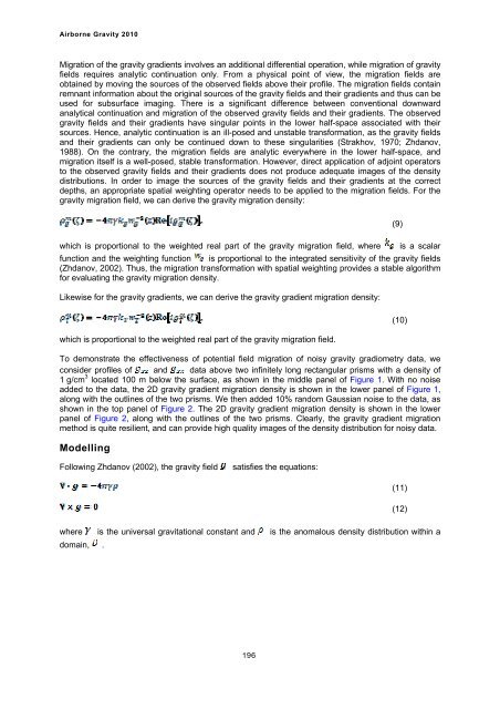
gravity migration field, we can derive the gravity migration density:
which is proportional to the weighted real part of the gravity migration field, where is a scalar
function and the weighting function is proportional to the integrated sensitivity of the gravity fields
(Zhdanov, 2002). Thus, the migration transformation with spatial weighting provides a stable algorithm
for evaluating the gravity migration density.
Likewise for the gravity gradients, we can derive the gravity gradient migration density:
which is proportional to the weighted real part of the gravity migration field.
To demonstrate the effectiveness of potential field migration of noisy gravity gradiometry data, we
consider profiles of and data above two infinitely long rectangular prisms with a density of
1 g/cm 3 located 100 m below the surface, as shown in the middle panel of Figure 1. With no noise
added to the data, the 2D gravity gradient migration density is shown in the lower panel of Figure 1,
along with the outlines of the two prisms. We then added 10% random Gaussian noise to the data, as
shown in the top panel of Figure 2. The 2D gravity gradient migration density is shown in the lower
panel of Figure 2, along with the outlines of the two prisms. Clearly, the gravity gradient migration
method is quite resilient, and can provide high quality images of the density distribution for noisy data.
Modelling
Following Zhdanov (2002), the gravity field satisfies the equations:
where is the universal gravitational constant and is the anomalous density distribution within a
domain, .
196
(9)
(10)
(11)
(12)