Airborne Gravity 2010 - Geoscience Australia

Airborne Gravity 2010
the full calculation with no grouping (i.e., subdivide at every step) and a value of one is generally a
crude approximation.
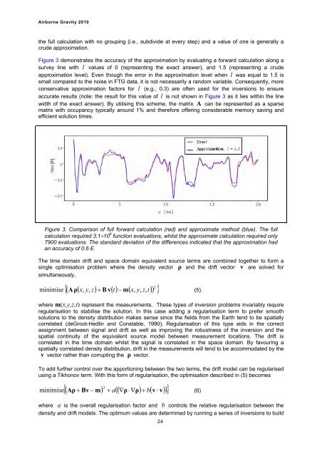
Figure 3 demonstrates the accuracy of the approximation by evaluating a forward calculation along a
survey line with l values of 0 (representing the exact answer), and 1.5 (representing a crude
approximation level). Even though the error in the approximation level when l was equal to 1.5 is
small compared to the noise in FTG data, it is not necessarily a random variable. Consequently, more
conservative approximation factors for l (e.g., 0.3) are often used for the inversions to ensure
accurate results (note: the result for this value of l is not shown in Figure 3 as it lies within the line
width of the exact answer). By utilising this scheme, the matrix A can be represented as a sparse
matrix with occupancy typically around 1% and therefore offering considerable memory saving and
efficient solution times.
Figure 3. Comparison of full forward calculation (red) and approximate method (blue). The full
calculation required 3.1�10 6 function evaluations, whilst the approximate calculation required only
7900 evaluations. The standard deviation of the differences indicated that the approximation had
an accuracy of 0.6 E.
The time domain drift and space domain equivalent source terms are combined together to form a
single optimisation problem where the density vector ρ and the drift vector v are solved for
simultaneously,
�� � � � � � ��
� 2
Aρ x, y,
z B v t � m x,
y,
z,
minimise � t
(5).
where m(x,y,z,t) represent the measurements. These types of inversion problems invariably require
regularisation to stabilise the solution. In this case adding a regularisation term to prefer smooth
solutions to the density distribution makes sense since the fields from the Earth tend to be spatially
correlated (deGroot-Hedlin and Constable, 1990). Regularisation of this type aids in the correct
assignment between signal and drift as well as improving the robustness of the inversion and the
spatial continuity of the equivalent source model between measurement locations. The drift is
correlated in the time domain whilst the signal is correlated in the space domain. By favouring a
spatially correlated density distribution, drift in the measurements will tend to be accommodated by the
v vector rather than corrupting the ρ vector.
To add further control over the apportioning between the two terms, the drift model can be regularised
using a Tikhonov term. With this form of regularisation, the optimisation described in (5) becomes
2
��Aρ�Bv � m�
� a���ρ��ρ��b�v�v���
minimise (6)
where a is the overall regularisation factor and b controls the relative regularisation between the
density and drift models. The optimum values are determined by running a series of inversions to build
24