Airborne Gravity 2010 - Geoscience Australia

Airborne Gravity 2010
elements) at each crossover point was chosen as the function to minimise. This method works quickly
and efficiently and follows the original philosophy exactly. It should be applied after all obvious
“corrugations” have been previously levelled, e.g., with methods similar to the heading correction or
compensation discussed above.
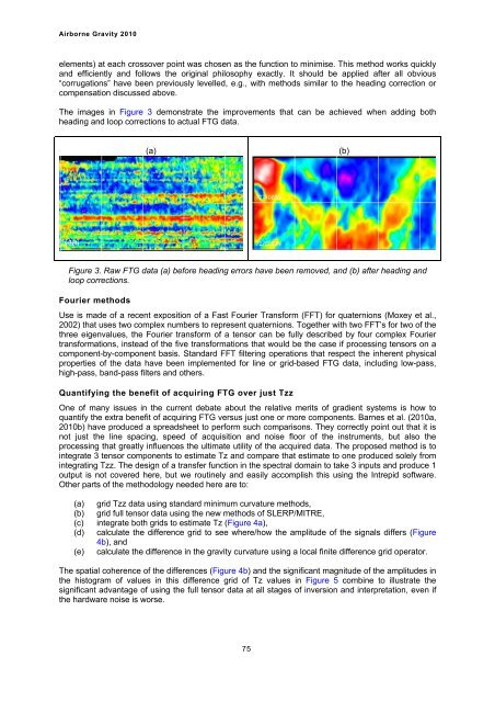
The images in Figure 3 demonstrate the improvements that can be achieved when adding both
heading and loop corrections to actual FTG data.
(a)
Figure 3. Raw FTG data (a) before heading errors have been removed, and (b) after heading and
loop corrections.
Fourier methods
Use is made of a recent exposition of a Fast Fourier Transform (FFT) for quaternions (Moxey et al.,
2002) that uses two complex numbers to represent quaternions. Together with two FFT’s for two of the
three eigenvalues, the Fourier transform of a tensor can be fully described by four complex Fourier
transformations, instead of the five transformations that would be the case if processing tensors on a
component-by-component basis. Standard FFT filtering operations that respect the inherent physical
properties of the data have been implemented for line or grid-based FTG data, including low-pass,
high-pass, band-pass filters and others.
Quantifying the benefit of acquiring FTG over just Tzz
One of many issues in the current debate about the relative merits of gradient systems is how to
quantify the extra benefit of acquiring FTG versus just one or more components. Barnes et al. (2010a,
2010b) have produced a spreadsheet to perform such comparisons. They correctly point out that it is
not just the line spacing, speed of acquisition and noise floor of the instruments, but also the
processing that greatly influences the ultimate utility of the acquired data. The proposed method is to
integrate 3 tensor components to estimate Tz and compare that estimate to one produced solely from
integrating Tzz. The design of a transfer function in the spectral domain to take 3 inputs and produce 1
output is not covered here, but we routinely and easily accomplish this using the Intrepid software.
Other parts of the methodology needed here are to:
(a) grid Tzz data using standard minimum curvature methods,
(b) grid full tensor data using the new methods of SLERP/MITRE,
(c) integrate both grids to estimate Tz (Figure 4a),
(d) calculate the difference grid to see where/how the amplitude of the signals differs (Figure
4b), and
(e) calculate the difference in the gravity curvature using a local finite difference grid operator.
The spatial coherence of the differences (Figure 4b) and the significant magnitude of the amplitudes in
the histogram of values in this difference grid of Tz values in Figure 5 combine to illustrate the
significant advantage of using the full tensor data at all stages of inversion and interpretation, even if
the hardware noise is worse.
75
(b)