Airborne Gravity 2010 - Geoscience Australia

Airborne Gravity 2010
(a)
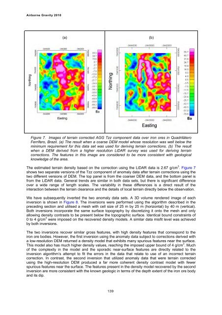
Figure 7. Images of terrain corrected AGG Tzz component data over iron ores in Quadrilátero
Ferrífero, Brazil. (a) The result when a coarse DEM model whose resolution was well below the
minimum requirement for this data set was used for deriving terrain corrections. (b) The result
when a DEM derived from a higher resolution LiDAR survey was used for deriving terrain
corrections. The features in this image are considered to be more consistent with geological
knowledge of the area.
The estimated terrain density based on the correction using the LiDAR data is 2.67 g/cm 3 . Figure 7
shows two separate versions of the Tzz component of anomaly data after terrain corrections using the
two different versions of DEM. The top panel is from the coarser DEM data, and the bottom panel is
from the LiDAR data. General trends are similar in both data sets, but there is significant difference
over a wide range of length scales. The variability in these differences is a direct result of the
interaction between the terrain clearance and the details of local terrain directly below the observation.
We have subsequently inverted the two anomaly data sets. A 3D volume rendered image of each
inversion is shown in Figure 8. The inversions were performed using the algorithm described in the
preceding section and utilised a mesh with cell size of 25 m by 25 m (horizontal) by 40 m (vertical).
Both inversions incorporate the same surface topography by discretizing it onto the mesh and only
allowing density contrasts to be present below the topographic surface. Identical bound constraints of
0 to 4 g/cm 3 were imposed on the recovered density models. A similar data misfit level was achieved
by both inversions.
The two inversions recover similar gross features, with high density features that correspond to the
iron ore bodies. However, the first inversion using the anomaly data subject to corrections derived with
a low-resolution DEM returned a density model that exhibits many spurious features near the surface.
This model also has much higher density values, reaching the imposed upper bound of 4 g/cm 3 . Much
of the complexity in the model and the sporadic near-surface features are directly related to the
inversion algorithm’s attempt to fit the errors in the data that relate to use of an incorrect terrain
correction. In contrast, the second inversion that utilized anomaly data that were terrain corrected
using the high-resolution DEM produced a far more coherent density contrast model with fewer
spurious features near the surface. The features present in the density model recovered by the second
inversion are more consistent with the known geologic in terms of the depth extent of the iron ore body
and its dip.
139
(b)