Airborne Gravity 2010 - Geoscience Australia

Airborne Gravity 2010
(a)
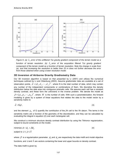
Figure 6. (a) L� error of the unfiltered Tzz gravity gradient component of the terrain model as a
function of terrain resolution. (b) L� error of the acquisition filtered Tzz gravity gradient
component of the terrain model as a function of terrain resolution. Note the change in scale from
(a), and that increasing the resolution to better than 20 m does not further decrease the error
from those obtained when using a lower resolution model.
3D Inversion of Airborne Gravity Gradiometry Data
Our 3D inversion algorithm is based on that presented by Li (2001) and utilizes the numerical
techniques outlined by Li and Oldenburg (2003). Assume gradiometer data are available at a set of
� T
observation points, d � ( d1,
d 2 , �,
d N ) , where N is the total number of data, which may contain
any number of the independent components or combinations of them. We discretize the density
distribution below the data area into contiguous prismatic cells. We assume each cell has a constant
density contrast, and these form the unknowns in the inverse problem. We denote the model as
T
M ) , , , ( �
� � �1
�2
� � , where M is the number of cells. With such a parameterization, the forward
modeling is given by a system of linear equations that relates the data to the model vector by a
sensitivity matrix G:
�
d � G , (3)
� �
and the element g ij of G quantify the contribution of the j'th cell to the i'th datum. The terms in the
sensitivity matrix are a function of the geometry of the discretization, and they can be calculated by
evaluating the integral in equation (2) over each rectangular cell.
We construct a minimum structure density contrast distribution by using the Tikhonov regularization,
subject to bound constraints on the model,
minimize � � �d
� ���
(4)
� � �
subject to a � � � b
where � is a regularization parameter, �d and �� are respectively the data misfit and model objective
functions, and a � and b � are vectors containing the lower and upper bounds on density contrast.
The data misfit is given by
137
(b)