Airborne Gravity 2010 - Geoscience Australia

Airborne Gravity 2010
reduce computer memory requirements and run times, can usually be accomplished without serious
loss of accuracy after terrain correction.
Effect of along-line filtering
Processing of gravity gradient data involves along-line low-pass filtering to suppress noise. A delicate
balance is required in order to achieve an improvement in S/N without seriously degrading resolution.
Detailed understanding of the along-line filtering is important for quantitative interpretation, since the
same filtering should be applied to calculated data. Unfortunately, the relevant information is not
always communicated by contractors.
If a “high resolution” terrain correction is applied to filtered data, artifacts will be introduced if the
accurate terrain response contains wavelengths shorter than the filter cut-off (Kass and Li, 2007). The
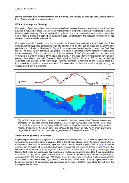
potential for confusion is illustrated in Figure 2, showing a north-south section through the Red Dog
model. The exact terrain-corrected Gzz profile (red) can be compared with the result of full resolution
terrain correction of filtered data (black). A terrain density of 2.67 g/cc was adopted, and Gzz was
computed at a uniform drape of 80 m above the ground. A low-pass filter with full pass for wavelengths
greater than 400 m, and with Gaussian bell roll-off to half amplitude at 300 m, was applied to
calculated Gzz profiles. Short wavelength “filtering artefacts” introduced in this fashion could be
interpreted as subsurface density variations. The anomalies can be substantial in amplitude, e.g., in
excess of 30 Eo in this example.
Figure 2. Comparison of exact terrain-corrected Gzz (red) with the result of full resolution terraincorrection
of low-pass filtered Gzz (black). Filter cut-off wavelength was 400 m. Data were
computed for a north-south section (178640E) across a simplified model of the Red Dog deposit,
Alaska. Densities in the lower panel are relative to the terrain density (2.67 g/cc). Elevations
range from 75 to 425 m, and vertical exaggeration is x2. The profile spans 1700 m.
Selection of quantity to interpret
Depending on the acquisition system, the interpreter will usually have two or more independent tensor
components, or combinations, to analyse. Gzz is the obvious choice, given its simple relationship to
causative bodies and its relatively large amplitude, hence usually superior S/N (Figure 3). While
examination of images of individual components, or combinations including tensor invariants, may be
beneficial for identification of stratigraphic or structural or mineralised trends (e.g., Mataragio and
Kieley, 2009), it is our experience that inversion of multiple components adds little if Gzz is available.
In contrast to any small gain in knowledge or confidence, inversion of multiple components is
computationally far more intensive. Moreover, there are traps when inverting multiple components:
simultaneous inversion of Gxx, Gyy, and Gzz will usually fail by virtue of linear dependence. Other
linear combinations of components are dependent to the extent that they can all be derived form the
same potential function.
81