Airborne Gravity 2010 - Geoscience Australia

Airborne Gravity 2010
The instrument operates at cryogenic temperatures (below 5 K), in order to minimize thermallyinduced
noise, and in order to make use of several useful properties of superconducting materials and
devices; e.g., the instrument employs the Paik transducer (Paik, 1976) to stably resolve motions of the
test-masses to better than 10 -13 m, enabling the instrument to measure gravity gradients less than 1 E.
The Paik transducer employs superconducting niobium test-masses, superconducting-wire inductive
coils, superconducting connecting wiring, and SQUID sensors.
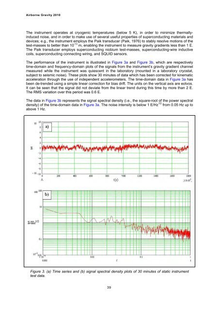
The performance of the instrument is illustrated in Figure 3a and Figure 3b, which are respectively
time-domain and frequency-domain plots of the signals from the instrument’s gravity gradient channel
measured while the instrument was quiescent in the laboratory (mounted in a laboratory cryostat,
subject to seismic noise). These plots show 30 minutes of data which has been corrected for kinematic
acceleration through the use of independent accelerometers. The time-domain data in Figure 3a has
been de-trended using a simple linear correction for bias drift. The units on the vertical axis are eotvos.
It can be seen that the signal did not deviate from the linear trend during this time by more than 2 E.
The RMS variation over this period was 0.6 E.
The data in Figure 3b represents the signal spectral density (i.e., the square-root of the power spectral
density) of the time-domain data in Figure 3a. The noise intensity is below 1 E/Hz 1/2 from 0.05 Hz up to
above 1 Hz.
Figure 3. (a) Time series and (b) signal spectral density plots of 30 minutes of static instrument
test data.
39