Airborne Gravity 2010 - Geoscience Australia
Airborne Gravity 2010 - Geoscience Australia
Airborne Gravity 2010 - Geoscience Australia
Create successful ePaper yourself
Turn your PDF publications into a flip-book with our unique Google optimized e-Paper software.
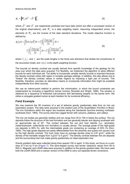
<strong>Airborne</strong> <strong>Gravity</strong> <strong>2010</strong><br />
� � 2<br />
o p<br />
� � W ( d � d ) , (5)<br />
d<br />
d<br />
2<br />
p<br />
where d � o<br />
and d � are respectively predicted and input data (which are often a processed version of<br />
the original observations), and W d is a data weighting matrix. Assuming independent errors, the<br />
elements of W d are the inverse of the data standard deviations. The model objective function is<br />
defined by<br />
2<br />
2 2 ��w(<br />
z)<br />
� �<br />
�� ( �)<br />
� � �w( z)<br />
��<br />
dv � lx<br />
� � dv<br />
x � �<br />
V<br />
V � � �<br />
(6)<br />
2<br />
2<br />
2 ��w(<br />
z)<br />
� � 2 ��w(<br />
z)<br />
� �<br />
ly<br />
� � dv � lz<br />
dv<br />
y<br />
� � � z �<br />
V � � �<br />
V � � �<br />
where l x , l y , and l z are the scale lengths in the three axis directions that dictate the smoothness of<br />
the recovered model, and w (z)<br />
is the depth weighting function.<br />
The bounds on density contrast are usually derived from specific knowledge of the geology for the<br />
area over which the data were acquired. For flexibility, we implement the algorithm to allow different<br />
bounds for each individual cell. The ability to incorporate variable density bounds is important because<br />
the density contrast varies with region in complex geologic settings. In addition, this also allows one to<br />
"freeze" the density contrast values in certain regions by imposing a tight pair of bounds. This<br />
flexibility, therefore, provides an alternative means to incorporate information that might be available<br />
independently from other sources.<br />
We use an interior-point method to perform the minimization, in which the bound constraints are<br />
implemented by including a logarithmic barrier function (Nocedal and Wright, 1999). The solution is<br />
obtained by a sequence of linearized sub-solutions with decreasing weights on the barrier term. We<br />
utilize a conjugate gradient solver at each iteration for its numerical efficiency.<br />
Field Example<br />
We now examine the 3D inversion of a set of airborne gravity gradiometry data from an iron ore<br />
exploration project. The data were acquired in the western part of the Quadrilátero Ferrífero in Brazil.<br />
The iron formations within the region are localized along the Gandarela Syncline trending northeastsouthwest<br />
(Dorr, 1965). The survey area has rugged terrain with canyons, plateaus, and valleys.<br />
The iron ore bodies are generally shallow and can range from 25 to 150 m below the surface. The ore<br />
deposits follow the structure of the host formation and are generally tabular and dipping southeast with<br />
an approximate dip of 25�. The contact between the ore and host itabirite (i.e., laminated,<br />
metamorphosed, oxide-facies iron formation) is usually abrupt. The average grade of the high-grade<br />
ore deposits is 66% Fe, with the intermediate grade ore containing an average of 63% Fe (Dorr,<br />
1965). The high-grade deposits are easily differentiated from the dolomitic and quartz-rich country rock<br />
by the high density contrast. The host rocks have an average density close to 2.67 g/cm 3 , while the<br />
density of the hematite ranges from 3 g/cm 3 to 5 g/cm 3 . The density contrast between the ore deposits<br />
and the surrounding host rock make gravity gradiometry an ideal exploration tool.<br />
<strong>Gravity</strong> gradient data were collected along lines spaced 100 m apart. In this study, we focus on a subarea<br />
of 4 km by 5 km (Figure 7). The semi-draped survey had terrain clearance values from 60 to<br />
500 m. Magnetic and LiDAR data were acquired in addition to the gravity gradient data. We have used<br />
both the LiDAR DEM and a coarser version of this DEM to carry out separate terrain corrections.<br />
138


