Airborne Gravity 2010 - Geoscience Australia

Airborne Gravity 2010
seen below, this is especially noticeable in regions of strong curvature of the potential field, or in other
words, where the geological features causing the field anomalies are located. Thus, an interpolation
method for tensors is required which takes their intrinsic physical properties into account.
Following the separation of concerns into amplitude and rotations, a means is sought for smoothly
interpolating rotations and combining this with amplitude estimation. As discussed above, unit
quaternions can be used to parameterize rotations. They form a 4D unit hypersphere and each point
on this hypersphere defines a rotation axis and a rotation angle. Thus, interpolated points lie along
geodesics, which are given by great circles, the analogue of straight line segments in the plane. The
interpolation of points along great circles is achieved by so-called spherical linear interpolation, or
“SLERP” (Shoemake 1995; Kuipers 1999). Currently, full tensor interpolation is implemented in the
Intrepid software as a triangle or 3-point interpolation algorithm. There is a patent on this development
(FitzGerald and Holstein, 2006).
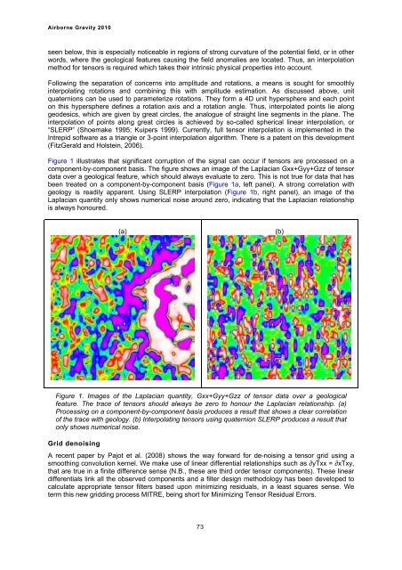
Figure 1 illustrates that significant corruption of the signal can occur if tensors are processed on a
component-by-component basis. The figure shows an image of the Laplacian Gxx+Gyy+Gzz of tensor
data over a geological feature, which should always evaluate to zero. This is not true for data that has
been treated on a component-by-component basis (Figure 1a, left panel). A strong correlation with
geology is readily apparent. Using SLERP interpolation (Figure 1b, right panel), an image of the
Laplacian quantity only shows numerical noise around zero, indicating that the Laplacian relationship
is always honoured.
(a)
Figure 1. Images of the Laplacian quantity, Gxx+Gyy+Gzz of tensor data over a geological
feature. The trace of tensors should always be zero to honour the Laplacian relationship. (a)
Processing on a component-by-component basis produces a result that shows a clear correlation
of the trace with geology. (b) Interpolating tensors using quaternion SLERP produces a result that
only shows numerical noise.
Grid denoising
A recent paper by Pajot et al. (2008) shows the way forward for de-noising a tensor grid using a
smoothing convolution kernel. We make use of linear differential relationships such as ∂yTxx = ∂xTxy,
that are true in a finite difference sense (N.B., these are third order tensor components). These linear
differentials link all the observed components and a filter design methodology has been developed to
calculate appropriate tensor filters based upon minimizing residuals, in a least squares sense. We
term this new gridding process MITRE, being short for Minimizing Tensor Residual Errors.
73
(b)