Airborne Gravity 2010 - Geoscience Australia

Airborne Gravity 2010
Because the line data do not sample the peak, the gridded values do not accurately reflect the true
peak. In Figure 6, the two curves match at the line locations every 200 m but differ between them.
When taken in 2 dimensions, these differences are what cause most of the problems. However, even
if there are differences, does this make any difference to the interpretability of the data?
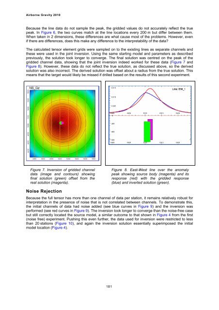
The calculated tensor element grids were sampled on to the existing lines as separate channels and
these were used in the joint inversion. Using the same starting model and parameters as described
previously, the solution took longer to converge. The final solution was centred on the peak of the
gridded channel data, showing that the joint inversion indeed worked for these data (Figure 7 and
Figure 8). However, these data do not reflect the true solution, as discussed above, so the derived
solution was also incorrect. The derived solution was offset about a radius from the true solution. This
means that the target would likely be missed if drilled based on the results of this second experiment.
Figure 7. Inversion of gridded channel
data (image and contours) showing
final solution (green) offset from the
real solution (magenta).
Noise Rejection
181
Figure 8. East-West line over the anomaly
peak showing source body (magenta) and its
response (red) with the gridded response
(blue) and inverted solution (green).
Because the full tensor has more than one channel of data per station, it remains relatively robust for
interpretation in the presence of noise that is not correlated between channels. To demonstrate this,
the initial channels of data had noise added (see blue curves in Figure 9) and the inversion was
performed (see red curves in Figure 9). The inversion took longer to converge than the noise-free case
but still correctly located the source model, a similar outcome to that shown in Figure 4 from the first
(noise free) experiment. Pushing this even further, the data used for inversion were restricted to less
than 20 stations (Figure 10), and again the inversion solution essentially superimposed the initial
model location (Figure 4).