Four degrees and beyond: the potential for a global ... - Amper

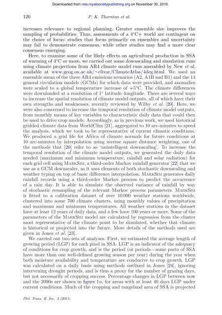
120 P. K. Thornton et al.
increases relevance to regional planning. Greater ensemble size improves the
sampling of probabilities. Thus, assessments of a 4 ◦ C+ world are contingent on
the choice of focus: studies that focus primarily on ensembles and uncertainty
may fail to demonstrate consensus, while other studies may find a more clear
consensus emerging.
Here, to examine some of the likely effects on agricultural production in SSA
of warming of 4 ◦ C or more, we carried out some downscaling and simulation runs
using climate projections from AR4 climate model runs assembled by New et al.
available at www.geog.ox.ac.uk/∼clivar/ClimateAtlas/4deg.html. We used an
ensemble mean of the three AR4 emissions scenarios (A2, A1B and B1) and the 14
general circulation models (GCMs) for which data were provided, and anomalies
were scaled to a global temperature increase of +5 ◦ C. The climate differences
were downloaded at a resolution of 1 ◦ latitude–longitude. There are several ways
to increase the spatial resolution of climate model outputs, all of which have their
own strengths and weaknesses, recently reviewed by Wilby et al. [20]. Here, we
were also concerned to increase the temporal resolution of climate model outputs,
from monthly means of key variables to characteristic daily data that could then
be used to drive crop models. Accordingly, as in previous work, we used historical
gridded climate data from WorldClim [21], aggregated to 10 arc-minutes to speed
the analysis, which we took to be representative of current climatic conditions.
We produced a grid file for Africa of climate normals for future conditions at
10 arc-minutes by interpolation using inverse square distance weighting, one of
the methods that [20] refer to as ‘unintelligent downscaling’. To increase the
temporal resolution of the climate model outputs, we generated the daily data
needed (maximum and minimum temperature, rainfall and solar radiation) for
each grid cell using MARKSIM, a third-order Markov rainfall generator [22] that we
use as a GCM downscaler, as it uses elements of both stochastic downscaling and
weather typing on top of basic difference interpolation. MARKSIM generates daily
rainfall records using a third-order Markov process to predict the occurrence
of a rain day. It is able to simulate the observed variance of rainfall by way
of stochastic resampling of the relevant Markov process parameters. MARKSIM
is fitted to a calibration dataset of over 10 000 weather stations worldwide,
clustered into some 700 climate clusters, using monthly values of precipitation
and maximum and minimum temperatures. All weather stations in the dataset
have at least 12 years of daily data, and a few have 100 years or more. Some of the
parameters of the MARKSIM model are calculated by regression from the cluster
most representative of the climate point to be simulated, whether that climate
is historical or projected into the future. More details of the methods used are
given in Jones et al. [23].
We carried out two sets of analyses. First, we estimated the average length of
growing period (LGP) for each pixel in SSA. LGP is an indicator of the adequacy
of conditions for crop growth, and is the period (or periods—some parts of SSA
have more than one well-defined growing season per year) during the year when
both moisture availability and temperature are conducive to crop growth. LGP
was calculated on a daily basis using methods outlined in Jones [24], ignoring
intervening drought periods, and is thus a proxy for the number of grazing days,
but not necessarily of cropping success. Percentage changes in LGP between now
and the 2090s are shown in figure 1a, for areas with at least 40 days LGP under
current conditions. Much of the cropping and rangeland area of SSA is projected
Phil. Trans. R. Soc. A (2011)
Downloaded from
rsta.royalsocietypublishing.org on November 30, 2010