Four degrees and beyond: the potential for a global ... - Amper
Four degrees and beyond: the potential for a global ... - Amper
Four degrees and beyond: the potential for a global ... - Amper

Create successful ePaper yourself
Turn your PDF publications into a flip-book with our unique Google optimized e-Paper software.
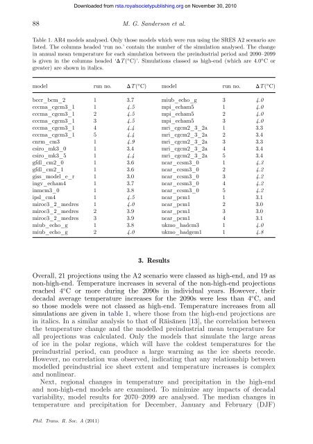
88 M. G. S<strong>and</strong>erson et al.<br />
Table 1. AR4 models analysed. Only those models which were run using <strong>the</strong> SRES A2 scenario are<br />
listed. The columns headed ‘run no.’ contain <strong>the</strong> number of <strong>the</strong> simulation analysed. The change<br />
in annual mean temperature <strong>for</strong> each simulation between <strong>the</strong> preindustrial period <strong>and</strong> 2090–2099<br />
is given in <strong>the</strong> columns headed ‘DT( ◦ C)’. Simulations classed as high-end (which are 4.0 ◦ Cor<br />
greater) are shown in italics.<br />
model run no. DT( ◦ C) model run no. DT( ◦ C)<br />
bccr_bcm_2 1 3.7 miub_echo_g 3 4.0<br />
cccma_cgcm3_1 1 4.5 mpi_echam5 1 4.0<br />
cccma_cgcm3_1 2 4.5 mpi_echam5 2 4.0<br />
cccma_cgcm3_1 3 4.5 mpi_echam5 3 4.0<br />
cccma_cgcm3_1 4 4.4 mri_cgcm2_3_2a 1 3.3<br />
cccma_cgcm3_1 5 4.4 mri_cgcm2_3_2a 2 3.4<br />
cnrm_cm3 1 4.9 mri_cgcm2_3_2a 3 3.3<br />
csiro_mk3_0 1 3.4 mri_cgcm2_3_2a 4 3.4<br />
csiro_mk3_5 1 4.4 mri_cgcm2_3_2a 5 3.4<br />
gfdl_cm2_0 1 3.6 ncar_ccsm3_0 1 4.3<br />
gfdl_cm2_1 1 3.6 ncar_ccsm3_0 2 4.2<br />
giss_model_e_r 1 3.0 ncar_ccsm3_0 3 4.2<br />
ingv_echam4 1 3.7 ncar_ccsm3_0 4 4.2<br />
inmcm3_0 1 3.8 ncar_ccsm3_0 5 4.2<br />
ipsl_cm4 1 4.5 ncar_pcm1 1 3.1<br />
miroc3_2_medres 1 4.0 ncar_pcm1 2 3.0<br />
miroc3_2_medres 2 3.9 ncar_pcm1 3 3.0<br />
miroc3_2_medres 3 3.9 ncar_pcm1 4 3.1<br />
miub_echo_g 1 3.8 ukmo_hadcm3 1 4.0<br />
miub_echo_g 2 4.0 ukmo_hadgem1 1 4.8<br />
3. Results<br />
Overall, 21 projections using <strong>the</strong> A2 scenario were classed as high-end, <strong>and</strong> 19 as<br />
non-high-end. Temperature increases in several of <strong>the</strong> non-high-end projections<br />
reached 4 ◦ C or more during <strong>the</strong> 2090s in individual years. However, <strong>the</strong>ir<br />
decadal average temperature increases <strong>for</strong> <strong>the</strong> 2090s were less than 4 ◦ C, <strong>and</strong><br />
so those models were not classed as high-end. Temperature increases from all<br />
simulations are given in table 1, where those from <strong>the</strong> high-end projections are<br />
in italics. In a similar analysis to that of Räisänen [13], <strong>the</strong> correlation between<br />
<strong>the</strong> temperature change <strong>and</strong> <strong>the</strong> modelled preindustrial mean temperature <strong>for</strong><br />
all projections was calculated. Only <strong>the</strong> models that simulate <strong>the</strong> large areas<br />
of ice in <strong>the</strong> polar regions, which will have <strong>the</strong> coldest temperatures <strong>for</strong> <strong>the</strong><br />
preindustrial period, can produce a large warming as <strong>the</strong> ice sheets recede.<br />
However, no correlation was observed, indicating that any relationship between<br />
modelled preindustrial ice sheet extent <strong>and</strong> temperature increases is complex<br />
<strong>and</strong> nonlinear.<br />
Next, regional changes in temperature <strong>and</strong> precipitation in <strong>the</strong> high-end<br />
<strong>and</strong> non-high-end models are examined. To minimize any impacts of decadal<br />
variability, model results <strong>for</strong> 2070–2099 are analysed. The median changes in<br />
temperature <strong>and</strong> precipitation <strong>for</strong> December, January <strong>and</strong> February (DJF)<br />
Phil. Trans. R. Soc. A (2011)<br />
Downloaded from<br />
rsta.royalsocietypublishing.org on November 30, 2010