Four degrees and beyond: the potential for a global ... - Amper

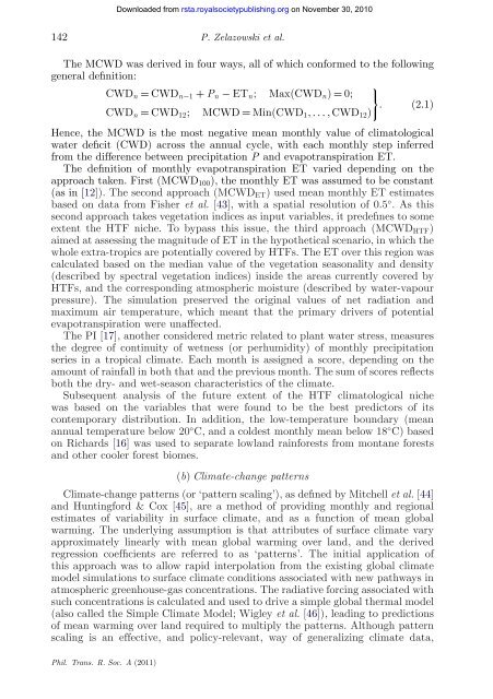
142 P. Zelazowski et al.
The MCWD was derived in four ways, all of which conformed to the following
general definition:
�
CWDn = CWDn−1 + Pn − ETn; Max(CWDn) = 0;
. (2.1)
CWDn = CWD12; MCWD = Min(CWD1, ..., CWD12)
Hence, the MCWD is the most negative mean monthly value of climatological
water deficit (CWD) across the annual cycle, with each monthly step inferred
from the difference between precipitation P and evapotranspiration ET.
The definition of monthly evapotranspiration ET varied depending on the
approach taken. First (MCWD100), the monthly ET was assumed to be constant
(as in [12]). The second approach (MCWDET) used mean monthly ET estimates
based on data from Fisher et al. [43], with a spatial resolution of 0.5 ◦ . As this
second approach takes vegetation indices as input variables, it predefines to some
extent the HTF niche. To bypass this issue, the third approach (MCWDHTF)
aimed at assessing the magnitude of ET in the hypothetical scenario, in which the
whole extra-tropics are potentially covered by HTFs. The ET over this region was
calculated based on the median value of the vegetation seasonality and density
(described by spectral vegetation indices) inside the areas currently covered by
HTFs, and the corresponding atmospheric moisture (described by water-vapour
pressure). The simulation preserved the original values of net radiation and
maximum air temperature, which meant that the primary drivers of potential
evapotranspiration were unaffected.
The PI [17], another considered metric related to plant water stress, measures
the degree of continuity of wetness (or perhumidity) of monthly precipitation
series in a tropical climate. Each month is assigned a score, depending on the
amount of rainfall in both that and the previous month. The sum of scores reflects
both the dry- and wet-season characteristics of the climate.
Subsequent analysis of the future extent of the HTF climatological niche
was based on the variables that were found to be the best predictors of its
contemporary distribution. In addition, the low-temperature boundary (mean
annual temperature below 20 ◦ C, and a coldest monthly mean below 18 ◦ C) based
on Richards [16] was used to separate lowland rainforests from montane forests
and other cooler forest biomes.
(b) Climate-change patterns
Climate-change patterns (or ‘pattern scaling’), as defined by Mitchell et al. [44]
and Huntingford & Cox [45], are a method of providing monthly and regional
estimates of variability in surface climate, and as a function of mean global
warming. The underlying assumption is that attributes of surface climate vary
approximately linearly with mean global warming over land, and the derived
regression coefficients are referred to as ‘patterns’. The initial application of
this approach was to allow rapid interpolation from the existing global climate
model simulations to surface climate conditions associated with new pathways in
atmospheric greenhouse-gas concentrations. The radiative forcing associated with
such concentrations is calculated and used to drive a simple global thermal model
(also called the Simple Climate Model; Wigley et al. [46]), leading to predictions
of mean warming over land required to multiply the patterns. Although pattern
scaling is an effective, and policy-relevant, way of generalizing climate data,
Phil. Trans. R. Soc. A (2011)
Downloaded from
rsta.royalsocietypublishing.org on November 30, 2010