Four degrees and beyond: the potential for a global ... - Amper

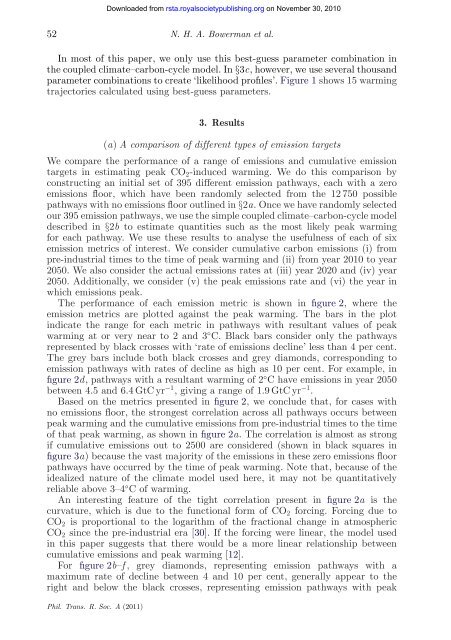
52 N. H. A. Bowerman et al.
In most of this paper, we only use this best-guess parameter combination in
the coupled climate–carbon-cycle model. In §3c, however, we use several thousand
parameter combinations to create ‘likelihood profiles’. Figure 1 shows 15 warming
trajectories calculated using best-guess parameters.
3. Results
(a) A comparison of different types of emission targets
We compare the performance of a range of emissions and cumulative emission
targets in estimating peak CO2-induced warming. We do this comparison by
constructing an initial set of 395 different emission pathways, each with a zero
emissions floor, which have been randomly selected from the 12 750 possible
pathways with no emissions floor outlined in §2a. Once we have randomly selected
our 395 emission pathways, we use the simple coupled climate–carbon-cycle model
described in §2b to estimate quantities such as the most likely peak warming
for each pathway. We use these results to analyse the usefulness of each of six
emission metrics of interest. We consider cumulative carbon emissions (i) from
pre-industrial times to the time of peak warming and (ii) from year 2010 to year
2050. We also consider the actual emissions rates at (iii) year 2020 and (iv) year
2050. Additionally, we consider (v) the peak emissions rate and (vi) the year in
which emissions peak.
The performance of each emission metric is shown in figure 2, where the
emission metrics are plotted against the peak warming. The bars in the plot
indicate the range for each metric in pathways with resultant values of peak
warming at or very near to 2 and 3 ◦ C. Black bars consider only the pathways
represented by black crosses with ‘rate of emissions decline’ less than 4 per cent.
The grey bars include both black crosses and grey diamonds, corresponding to
emission pathways with rates of decline as high as 10 per cent. For example, in
figure 2d, pathways with a resultant warming of 2 ◦ C have emissions in year 2050
between 4.5 and 6.4 GtC yr −1 , giving a range of 1.9 GtC yr −1 .
Based on the metrics presented in figure 2, we conclude that, for cases with
no emissions floor, the strongest correlation across all pathways occurs between
peak warming and the cumulative emissions from pre-industrial times to the time
of that peak warming, as shown in figure 2a. The correlation is almost as strong
if cumulative emissions out to 2500 are considered (shown in black squares in
figure 3a) because the vast majority of the emissions in these zero emissions floor
pathways have occurred by the time of peak warming. Note that, because of the
idealized nature of the climate model used here, it may not be quantitatively
reliable above 3–4 ◦ C of warming.
An interesting feature of the tight correlation present in figure 2a is the
curvature, which is due to the functional form of CO2 forcing. Forcing due to
CO2 is proportional to the logarithm of the fractional change in atmospheric
CO2 since the pre-industrial era [30]. If the forcing were linear, the model used
in this paper suggests that there would be a more linear relationship between
cumulative emissions and peak warming [12].
For figure 2b–f , grey diamonds, representing emission pathways with a
maximum rate of decline between 4 and 10 per cent, generally appear to the
right and below the black crosses, representing emission pathways with peak
Phil. Trans. R. Soc. A (2011)
Downloaded from
rsta.royalsocietypublishing.org on November 30, 2010