Four degrees and beyond: the potential for a global ... - Amper

emissions (GtC yr –1 )
14
12
10
8
6
4
2
Cumulative carbon emissions 49
0
0
1900 2000 2100 2200 2300 2400 2500
year
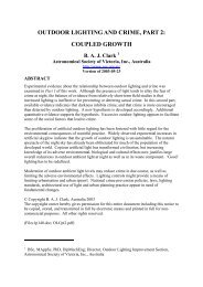
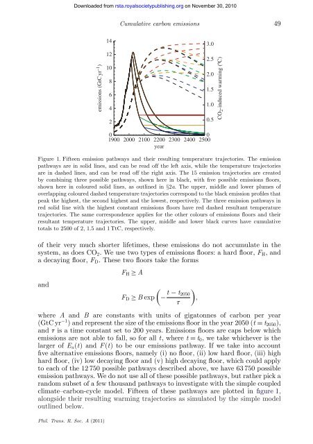
Figure 1. Fifteen emission pathways and their resulting temperature trajectories. The emission
pathways are in solid lines, and can be read off the left axis, while the temperature trajectories
are in dashed lines, and can be read off the right axis. The 15 emission trajectories are created
by combining three possible pathways, shown here in black, with five possible emissions floors,
shown here in coloured solid lines, as outlined in §2a. The upper, middle and lower plumes of
overlapping coloured dashed temperature trajectories correspond to the black emission profiles that
peak the highest, the second highest and the lowest, respectively. The three emission pathways in
red solid line with the highest constant emissions floors have red dashed resultant temperature
trajectories. The same correspondence applies for the other colours of emissions floors and their
resultant temperature trajectories. The upper, middle and lower black curves have cumulative
totals to 2500 of 2, 1.5 and 1 TtC, respectively.
of their very much shorter lifetimes, these emissions do not accumulate in the
system, as does CO2. We use two types of emissions floors: a hard floor, FH, and
a decaying floor, FD. These two floors take the forms
and
FH ≥ A
� �
t − t2050
FD ≥ B exp − ,
t
where A and B are constants with units of gigatonnes of carbon per year
(GtC yr −1 ) and represent the size of the emissions floor in the year 2050 (t = t2050),
and t is a time constant set to 200 years. Emissions floors are caps below which
emissions are not able to fall, so for all t, where t = t0, we take whichever is the
larger of Ea(t) and F(t) to be our emissions pathway. If we take into account
five alternative emissions floors, namely (i) no floor, (ii) low hard floor, (iii) high
hard floor, (iv) low decaying floor and (v) high decaying floor, which could apply
to each of the 12 750 possible pathways described above, we have 63 750 possible
emission pathways. We do not use all of these possible pathways, but rather pick a
random subset of a few thousand pathways to investigate with the simple coupled
climate–carbon-cycle model. Fifteen of these pathways are plotted in figure 1,
alongside their resulting warming trajectories as simulated by the simple model
outlined below.
Phil. Trans. R. Soc. A (2011)
Downloaded from
rsta.royalsocietypublishing.org on November 30, 2010
3.0
2.5
2.0
1.5
1.0
0.5
CO 2-induced warming (ºC)