- Page 2 and 3:
Proceedings of the International Co
- Page 4 and 5:
vw:. PREFACE Dunng a time when eart
- Page 6 and 7:
OPENING ADDRESS By Prof. Yuchen Liu
- Page 8 and 9:
Vll scientific support in our call
- Page 10 and 11:
IX INTERNATIONAL ADVISORY COMMITTEE
- Page 12 and 13:
XI Engineering Seismology and Geote
- Page 14 and 15:
Xlll Progress in the Seismic Design
- Page 16 and 17:
XV Crustal Deformation Measurement
- Page 19 and 20:
Proceedings of the International Co
- Page 21 and 22:
Legal Impediments There are many im
- Page 23:
expectation of (i) expanding the fr
- Page 26 and 27:
10 Some applications of wireless te
- Page 28 and 29:
12 Smart Materials Smart materials,
- Page 30 and 31:
14 research and education in a mult
- Page 33 and 34:
Proceedings of the International Co
- Page 35 and 36:
19 On September 16, 1994, buildings
- Page 37 and 38:
21 Some people were injured while t
- Page 39 and 40:
23 tallest buildings in Hong Kong w
- Page 41 and 42:
25 Figure 12. Tsim Sha Tsui East an
- Page 43 and 44:
27 OTHER ONGOING WORKS Soil-pile-st
- Page 45 and 46:
29 Figure 18. The pounding experime
- Page 47 and 48:
31 ACKNOWLEDGMENTS The writers are
- Page 49 and 50:
Proceedings of the International Co
- Page 51 and 52:
35 Table 1. Records Used in the Dev
- Page 53 and 54:
37 Date 8/19/1976 10/5/1977 12/16/1
- Page 55 and 56:
39 (2) Here Y is the ground motion
- Page 57 and 58:
41 1 2 3 4567810 20 3040 SO 100 200
- Page 59 and 60:
43 of the resultant horizontal comp
- Page 61 and 62:
45 200 006 005 004 003 002 Rock, Mw
- Page 63 and 64:
47 en o_ KOCAELI DATA (Random Hor C
- Page 65:
Atkinson G.M., Boore D.M., Some Com
- Page 68 and 69:
52 BACKGROUND AND SCOPES In order t
- Page 70 and 71:
configurations of cylinder, and it
- Page 72 and 73:
l 56 X xT / ^ V^—^E-^/i / X\ - yX
- Page 74 and 75:
58 59-74 (in Japanese) [7] ISHIKAWA
- Page 76 and 77:
60 accuracy and efficiency, have no
- Page 78 and 79:
62 f •c J — c. p «3 no Fig. 2
- Page 80 and 81:
64 VARIOUS TESTS AND DISSEMINATION
- Page 82 and 83:
66 response.. The post-earthquake i
- Page 85 and 86:
Proceedings of the International Co
- Page 87 and 88:
71 with the potential for self-diag
- Page 89 and 90:
73 Semi-active Hydraulic (SHD) Cont
- Page 91 and 92:
75 Table 1 Buildings currently unde
- Page 93 and 94:
77 and the inside of the damper cyl
- Page 95 and 96:
79 Figure 16. MR damper installatio
- Page 97 and 98:
81 sensors. New algorithms must be
- Page 99 and 100:
83 Kobon T. (1998). Mission and per
- Page 101 and 102:
Proceedings of the International Co
- Page 103 and 104:
87 for a period range less than 3.0
- Page 105 and 106:
89 tens or more than a hundred acce
- Page 107 and 108:
91 In order to validate the conclus
- Page 109 and 110:
93 Distance (km) """"--^Acc. (g) Ma
- Page 111 and 112:
95 CONCLUSION In this paper the imp
- Page 113:
ENGINEERING SEISMOLOGY AND GEOTECHN
- Page 116 and 117:
100 analyses. This paper reviews th
- Page 118 and 119:
102 A comparison of spectral amplit
- Page 120 and 121:
104 the high speed with which FFT c
- Page 122 and 123:
106 8. Gold, B. and C.M. Rader (197
- Page 124 and 125:
108 Displacement Curves", Dept. of
- Page 126 and 127:
I 000,000 100,000 Number of uniform
- Page 128 and 129:
Response and Fourier Spectra of Dig
- Page 130 and 131:
114 10 3 10 2 r | I lll| I | I | I
- Page 132 and 133:
116 analysis. Other techniques incl
- Page 134 and 135:
It has been found that G max applie
- Page 136 and 137:
120 PALEOLIQUEFACTION STUDIES IN ME
- Page 138 and 139:
Jardine, R.J., Potts, D.M., StJohn,
- Page 140 and 141:
124 has received more attention. In
- Page 142 and 143:
126 and log A tQ (/) is the mean so
- Page 144 and 145:
128 O 10 s Frequency (Hz) Frequency
- Page 146 and 147:
130 geometrical coefficient is near
- Page 148 and 149:
132 optimizing method in many engin
- Page 150 and 151:
134 Type-2 Fig.5 Three dimensional
- Page 152 and 153:
136 plane plane sliding x-z section
- Page 155 and 156:
Proceedings of the International Co
- Page 157 and 158:
141 1. System Definition define sys
- Page 159 and 160:
143 f«l-.J WJjfc >. « Relations -
- Page 161 and 162:
145 DS-5 Response Simulation across
- Page 163 and 164:
147 CM 1 CM 2 CM 3 CM-4 CM-5 CM-6 H
- Page 165 and 166:
Proceedings of the International Co
- Page 167 and 168:
151 Number of Pixels (Frequency) Th
- Page 169 and 170:
153 Red: possible impacted areas Gr
- Page 171 and 172:
155 Low reliability -(water-reflect
- Page 173 and 174:
Proceedings of the International Co
- Page 175 and 176:
Modem or Router Dial-up ISP The Int
- Page 177 and 178:
from observed images Fig 5 shows th
- Page 179 and 180:
163 Picked up building from image p
- Page 181 and 182:
Proceedings of the International Co
- Page 183 and 184:
167 evaluated by Seed's approximate
- Page 185 and 186:
169 R(z,N)is reached to 1 or more,
- Page 187:
171 subsoil and combined with the n
- Page 190 and 191:
174 defined target. Performance-bas
- Page 192 and 193:
176 (probability of being in or exc
- Page 194 and 195:
178 start to dominate the hazard at
- Page 196 and 197:
180 MAX STORY DUCTILITY vs NORM. ST
- Page 199 and 200:
Proceedings of the International Co
- Page 201 and 202:
185 Decision Making Support Tool' U
- Page 203 and 204:
Proceedings of the International Co
- Page 205 and 206:
189 31 Array Liujiaxia Reservoir Ar
- Page 207 and 208:
191 IV STATION YM kCED INTERVALS OF
- Page 209 and 210:
193 at different stations, the diff
- Page 211 and 212:
Proceedings of the International Co
- Page 213 and 214:
197 PROBLEMS AND CHALLENGES Earthqu
- Page 215 and 216:
199 Database s*n/ar_- ^ " Applicati
- Page 217 and 218:
201 o Fig. 7 VRML authoring - model
- Page 219:
SMART MATERIALS AND SMART STRUCTURE
- Page 223 and 224:
Proceedings of the International Co
- Page 225 and 226:
209 vector of measured control forc
- Page 227 and 228:
211 To examine the effect of the co
- Page 229 and 230:
213 from Fig. 2, we can get the res
- Page 231 and 232:
Proceedings of the Intel-national C
- Page 233 and 234:
217 where gj^i = g(X fcTl , F^+^it
- Page 235 and 236:
219 3 360 Deg. Fault Normal (Jan. 1
- Page 237 and 238:
221 Earthquake Sylmar 90 Sylinar 90
- Page 239 and 240:
Proceedings of the International Co
- Page 241 and 242:
225 0.6965, and 0.7094 Hz, which ar
- Page 243 and 244:
227 Two displacement sensors are po
- Page 245 and 246:
229 14% to 45% (under El Centre ear
- Page 247 and 248:
Proceedings of the International Co
- Page 249 and 250:
233 g ^ w (4) Notice that the stabi
- Page 251 and 252:
235 modes. An energy drop will be o
- Page 253 and 254:
237 PPF controller. The second mode
- Page 255 and 256:
Proceedings of the International Co
- Page 257 and 258:
241 In order to determine the appar
- Page 259 and 260:
243 RESULTS AND DISCUSSIONS Figure
- Page 261 and 262:
245 100 150 200 250 300 Magnetic Fl
- Page 263 and 264:
Proceedings of the International Co
- Page 265 and 266:
249 WOLFE, MASRI, CAFFREY Synthetic
- Page 267 and 268:
251 WOLFE, MASRI, CAFFREY Transform
- Page 269 and 270:
253 WOLFE MASRI,CAFFREY in parallel
- Page 271:
STRUCTURAL ANALYSIS AND DESIGN
- Page 274 and 275:
258 separating the above three effe
- Page 276 and 277:
260 200 300 400 SHAKE Computed RSD^
- Page 278 and 279:
262 where H b is the building heigh
- Page 280 and 281:
264 6. ACKNOWLEDGEMENTS The work de
- Page 282 and 283:
266 The objectives of this paper pr
- Page 284 and 285:
268 The comparison between abovemen
- Page 286 and 287:
270 determine the span of the state
- Page 288 and 289:
the assumption of the bi-linear for
- Page 290 and 291:
274 There are several outstanding e
- Page 292 and 293:
276 buildings with different concre
- Page 294 and 295:
278 160,000 - 140,000 _^ d Concrete
- Page 296 and 297:
280 responded in a fairly similar m
- Page 298 and 299:
282 CONCLUSIONS In this paper, the
- Page 300 and 301:
284 Li B, Park, R. and Tanaka, H. (
- Page 302 and 303:
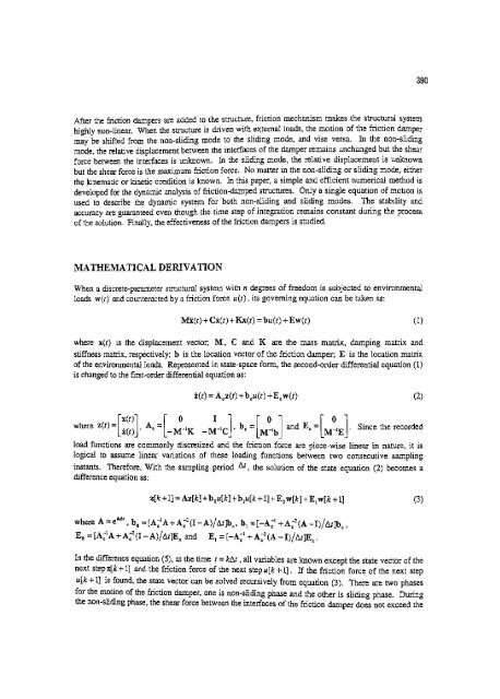
For simplicity, a linear distributi
- Page 304 and 305:
equation can be re- written as: 288
- Page 306 and 307:
290 DESIGN BASE SHEAR Equating the
- Page 308 and 309:
292 by using the computer program S
- Page 310 and 311:
294 mutation. Elitist strategy mean
- Page 312 and 313:
296 2.3 Premature Judgment and Comb
- Page 314 and 315:
298 (3) F 3 : De Jone's F 5 3 (Shek
- Page 316 and 317:
300 3.3 Test Conclusions From the t
- Page 318 and 319:
30; excitation. Also, the software
- Page 320 and 321:
304 concrete frames as documented i
- Page 322 and 323:
30€ NEURAL NETWORKS Development I
- Page 324 and 325:
308 ACKNOWLEDGEMENTS The research r
- Page 326 and 327:
310 In order to ensure the entire s
- Page 328 and 329:
312 Examples of Seismic Design In K
- Page 330 and 331:
314 earthquake load can be reduced
- Page 333 and 334:
Proceedings of the Intel national C
- Page 335 and 336:
319 broken. Therefore, joint elemen
- Page 337 and 338:
321 the highest probability to get
- Page 339 and 340:
Proceedings of the International Co
- Page 341 and 342:
325 DESIGN SPECIFICATIONS Overview
- Page 343 and 344:
327 Strength Degradation The streng
- Page 345 and 346:
I 329 file £dit Vww Select Constru
- Page 347 and 348:
Proceedings of the International Co
- Page 349 and 350:
333 (1) (2) Where f t and _/£ are
- Page 351 and 352:
335 JL dalt (10) Where Solution of
- Page 353 and 354:
337 Fig.9 Distribution of first pri
- Page 355 and 356: Proceedings of the International Co
- Page 357 and 358: 341 DISPLACMENT-BASED NSF In this p
- Page 359 and 360: 343 Define the displacement of the
- Page 361 and 362: 345 EXAMPLE The nonlinear static an
- Page 363: 347 REFERENCE Code for seismic desi
- Page 366 and 367: 350 including Hong Kong are conside
- Page 368 and 369: 352 structural engineers. Although
- Page 370 and 371: 354 4) Structural characteristics R
- Page 372 and 373: 356 maintain economy of design but
- Page 374 and 375: 358 R C3&OC11 L8C34 USC3 •••
- Page 377 and 378: Proceedings of the International Co
- Page 379 and 380: 363 DISPLACEMENT CALCULATION FOR GR
- Page 381 and 382: 365 As shown in the figure, a model
- Page 383 and 384: 367 history of a design earthquake
- Page 385 and 386: Proceedings of the International Co
- Page 387 and 388: 371 reflects the structure's useful
- Page 389 and 390: 373 have a membership degree betwee
- Page 391 and 392: 375 of initialization of structure,
- Page 393: 377 REFERENCE Zadeh, L A (1965), "F
- Page 397 and 398: Proceedings of the International Co
- Page 399 and 400: .0,(r+l,,)] (0 + A (3) 383 -l.y)] (
- Page 401 and 402: 385 The first example is come from
- Page 403 and 404: 387 REFERENCES Leroueil, S. (2001).
- Page 405: Proceedings of the International Co
- Page 409 and 410: 393 the stiffness of the bracing an
- Page 411 and 412: 395 splacemen (m) Bared —Braced/D
- Page 413 and 414: Proceedings of the International Co
- Page 415 and 416: 399 Figure 1: Two-surface Model Def
- Page 417 and 418: 401 time, one must integrate over t
- Page 419 and 420: 403 CONCLUSIONS In the previous sec
- Page 421 and 422: Proceedings of the International Co
- Page 423 and 424: 407 Response Control by Magneto-Rhe
- Page 425 and 426: 409 s e a ooo j| soo y 0 c l83Hz ,5
- Page 427 and 428: 411 *fU O A 20 7 HA I , 2 4A .'.-%-
- Page 429 and 430: Proceedings of the International Co
- Page 431 and 432: 415 Wind Velocity (t J Relative Dis
- Page 433 and 434: 417 Fig. 5 4ttractor (time lag=l) F
- Page 435: 419 concluded that the real time re
- Page 438 and 439: 422 (LQR/LQG), H M and the instanta
- Page 440 and 441: 424 damping ratio provided by the c
- Page 442 and 443: 426 by Eqn. 2.9 and Eqn. 2.12, resp
- Page 444 and 445: 428 Fig.5.4 shows the comparison of
- Page 446 and 447: Innovation is driving control devic
- Page 448 and 449: 432 STRUCTURAL ENERGY DURING VIBRAT
- Page 450 and 451: 434 Equilibrium Price of Power With
- Page 452 and 453: 436 CONCLUSION The scope of this re
- Page 454 and 455: 438 The effectiveness of the seismi
- Page 456 and 457:
440 anti-symmetnc mode excited by t
- Page 458 and 459:
442 Base Isolation System The base
- Page 460 and 461:
444 each member along or adjacent t
- Page 462 and 463:
446 2 PROJECT PARTICIPANTS Concerni
- Page 464 and 465:
448 3.1.2 Investigations at Seyhan
- Page 466 and 467:
450 Fig. 4.2: principle drawing of
- Page 468 and 469:
452 no TMD — TMD with optimal tun
- Page 470 and 471:
454 In this paper, a stochastic opt
- Page 472 and 473:
456 The dynamical programming equat
- Page 474 and 475:
458 control strategy. Model reducti
- Page 476 and 477:
460 (AMDs) and the proposed control
- Page 479 and 480:
Proceedings of the International Co
- Page 481 and 482:
465 Specimen 1 Specimen 1 represent
- Page 483 and 484:
467 increased the beam moment stren
- Page 485 and 486:
469 3 4@8 ~T / C 4 #5 #3 stirrups 8
- Page 487 and 488:
Proceedings of the International Co
- Page 489 and 490:
473 Phase 2: The sliding of the bot
- Page 491 and 492:
475 4.2 Effect of Coefficient of Fr
- Page 493 and 494:
477 -ZETA=Q 05 -ZETA=010 -ZETA=015
- Page 495:
479 031 en 03 0029 P |Q 28 ~*—MR=
- Page 498 and 499:
482 stiffness or coefficient of vis
- Page 500 and 501:
484 solved for the Hamilton Jacobi-
- Page 502 and 503:
486 posed to be the accelerations o
- Page 504 and 505:
488 vlaxacccleiation [my O O O O
- Page 506 and 507:
490 INTRODUCTION In recent years, t
- Page 508 and 509:
492 Since earthquake motion has bee
- Page 510 and 511:
494 confirmed in the X direction. B
- Page 512 and 513:
496 yielding metallic dampers, and
- Page 514 and 515:
498 where the coefficients a m and
- Page 516 and 517:
500 modal damping ratio of 2% in ea
- Page 518 and 519:
502 CONCLUDING REMARKS The paper re
- Page 520 and 521:
504 semi-active and hybrid control
- Page 522 and 523:
506 Iiz2i(t)l
- Page 524 and 525:
508 defined as 114 - [ J* [•] 2 d
- Page 526 and 527:
Spencer, B.F., Jr. and Sain, M.K. (
- Page 528 and 529:
512 with the rapid success of seism
- Page 530 and 531:
Figure 3 summarizes the static push
- Page 532 and 533:
CONCLUSIONS 516 This paper presents
- Page 534 and 535:
518 1 OS h : 0 6 5 5 04 Transverse
- Page 536 and 537:
520 TABLE 1 REPRESENTATIVE MULTISTO
- Page 538 and 539:
522 obtained by simply averaging a
- Page 540 and 541:
524 levels of peak ground accelerat
- Page 542 and 543:
526 8 CONCLUSIONS This paper gives
- Page 545 and 546:
Proceedings of the International Co
- Page 547 and 548:
531 350.6m 142.7m .0130') i (468')
- Page 549 and 550:
533 cation corresponds to a node of
- Page 551 and 552:
535 listed separately. Vertical mod
- Page 553 and 554:
Proceedings of the International Co
- Page 555 and 556:
539 in which H = [H(t l ), H(t 2 ),
- Page 557 and 558:
541 identification results of struc
- Page 559 and 560:
543 history to be polluted. In the
- Page 561:
Proceedings of the International Co
- Page 564 and 565:
548 environment constraints and the
- Page 566 and 567:
550 where F is the fundamental matr
- Page 568 and 569:
552 drift ratio was determined as Y
- Page 570 and 571:
554 were observed in the vision-sys
- Page 572 and 573:
556 The most well-known Bayesian so
- Page 574 and 575:
558 achieved by the EKF estimates I
- Page 576 and 577:
560 0 2 4 5 3 10 12 14 16 18 20 0 2
- Page 578 and 579:
562 CONCLUSION In this study, the r
- Page 580 and 581:
564 Figure 1 - Prototype wireless s
- Page 582 and 583:
566 will vary from that of the ARX
- Page 584 and 585:
568 A 11 25" 11 25" 1 T 1 11 25* !
- Page 586 and 587:
570 CONCLUSION The realization of a
- Page 588 and 589:
572 the structural response and ret
- Page 590 and 591:
574 The ratios of base shear at dif
- Page 592 and 593:
576 SECTION A-A COLUMN DETAIL AT TO
- Page 594 and 595:
578 Stress Strain Fig. 6 Superelast
- Page 596 and 597:
580 Genetic Algorithm(GA) and the M
- Page 598 and 599:
582 IDENTIFICATION ALGORITHM State
- Page 600 and 601:
584 the simulated structural respon
- Page 602 and 603:
586 GA-MCF, the number of particles
- Page 604 and 605:
588 instrumentation to monitor and
- Page 606 and 607:
590 If we compare this peak value w
- Page 608 and 609:
592 2.3 Sampling rate Structural mo
- Page 610 and 611:
594 Any remote station that has the
- Page 612 and 613:
596 or receives environmental infor
- Page 614 and 615:
598 Comparisons of Proposed E-Monit
- Page 616 and 617:
600 LCD display Earthquake Warning
- Page 619 and 620:
Proceedings of the International Co
- Page 621 and 622:
605 Kishwaukee River Bridge consist
- Page 623 and 624:
607 the table, the monthly maximum
- Page 625 and 626:
609 3.2 L VDTData Analysis LVDT sen
- Page 627 and 628:
Proceedings of the International Co
- Page 629 and 630:
structural response energy with fre
- Page 631 and 632:
615 Table 1: Fundamental natural fr
- Page 633 and 634:
617 JUSTS rs s." WUUR. 4 20O2 IS 44
- Page 635 and 636:
1-1 INDEX OF CONTRIBUTORS Volumes I
- Page 637:
Ths OOO F X ^s dje foe return 01 ^e