CMOS Optical Preamplifier Design Using Graphical Circuit Analysis

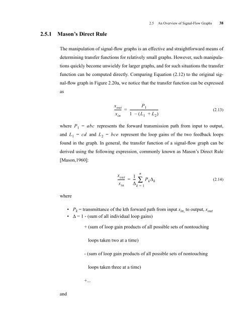
2.5.1 Mason’s Direct Rule
2.5 An Overview of Signal-Flow Graphs 38
The manipulation of signal-flow graphs is an effective and straightforward means of
determining transfer functions for relatively small graphs. However, such manipula-
tions quickly become unwieldy for larger graphs, and for such situations the transfer
function can be computed directly. Comparing Equation (2.12) to the original sig-
nal-flow graph in Figure 2.20a, we notice that the transfer function can be expressed
as
(2.13)
where = abc represents the forward transmission path from input to output,
and = cd and L2 = bce represent the loop gains of the two feedback loops
found in the graph. In general, the transfer function of a signal-flow graph can be
derived using the following expression, commonly known as Mason’s Direct Rule
[Mason,1960]:
where
and
L 1
P 1
• P k = transmittance of the kth forward path from input x in, to output, x out
• ∆ = 1 - (sum of all individual loop gains)
+ (sum of loop gain products of all possible sets of nontouching
loops taken two at a time)
- (sum of loop gain products of all possible sets of nontouching
+...
x out
--------
x in
x out
x in
loops taken three at a time)
P 1
= ----------------------------------
1 – ( L1 + L2) 1
-------- =
-- ∑ Pk∆ k
∆
n
k = 1
(2.14)