3D Time-of-flight distance measurement with custom - Universität ...

36 CHAPTER 2
mentioned before. The demodulation result for the measurement signal is then
falsified due to frequency dispersion by:
⎛ T ⎞
sinc⎜2π
⋅ ∆f
⋅
w
⎟
Equation 2.21
⎝ 2 ⎠
With TW=observation window/ integration time and ∆f=difference frequency of
measurement and spurious signal.
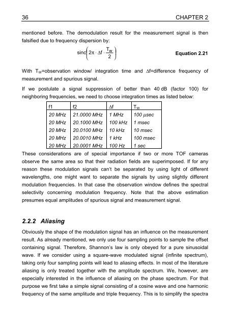
If we postulate a signal suppression of better than 40 dB (factor 100) for
neighboring frequencies, we need to choose integration times as listed below:
f1 f2 ∆f TW
20 MHz 21.0000 MHz 1 MHz 100 µsec
20 MHz 20.1000 MHz 100 kHz 1 msec
20 MHz 20.0100 MHz 10 kHz 10 msec
20 MHz 20.0010 MHz 1 kHz 100 msec
20 MHz 20.0001 MHz 100 Hz 1 sec
These considerations are of special importance if two or more TOF cameras
observe the same area so that their radiation fields are superimposed. If for any
reason these modulation signals can’t be separated by using light of different
wavelengths, one might want to separate the signals by using slightly different
modulation frequencies. In that case the observation window defines the spectral
selectivity concerning modulation frequency. Note that the above estimation
presumes equal amplitudes of spurious signal and measurement signal.
2.2.2 Aliasing
Obviously the shape of the modulation signal has an influence on the measurement
result. As already mentioned, we only use four sampling points to sample the offset
containing signal. Therefore, Shannon’s law is only obeyed for a pure sinusoidal
wave. If we consider using a square-wave modulated signal (infinite spectrum),
taking only four sampling points will lead to aliasing effects. In most of the literature
aliasing is only treated together with the amplitude spectrum. We, however, are
especially interested in the influence of aliasing on the phase spectrum. For that
purpose we first take a simple signal consisting of a cosine wave and one harmonic
frequency of the same amplitude and triple frequency. This is to simplify the spectra