THÈSE Estimation, validation et identification des modèles ARMA ...

Chapitre 3. Estimating the asymptotic variance of LSE of weak VARMA models 94
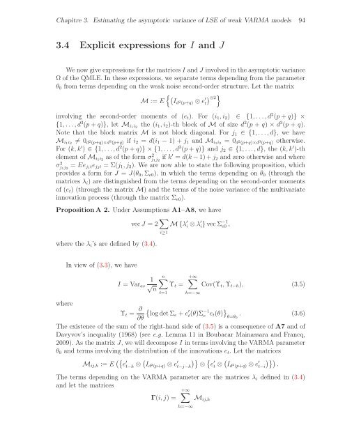
3.4 Explicit expressions for I and J
We now give expressions for the matricesI andJ involved in the asymptotic variance
Ω of the QMLE. In these expressions, we separate terms depending from the parameter
θ0 from terms depending on the weak noise second-order structure. Let the matrix
M := E
Id 2 (p+q) ⊗e ′
⊗2
t
involving the second-order moments of (et). For (i1,i2) ∈ {1,...,d 2 (p+q)} ×
{1,...,d 3 (p+q)}, let Mi1i2 the (i1,i2)-th block of M of size d 2 (p + q) × d 3 (p + q).
Note that the block matrix M is not block diagonal. For j1 ∈ {1,...,d}, we have
Mi1i2 = 0 d 2 (p+q)×d 3 (p+q) if i2 = d(i1 − 1) + j1 and Mi1i2 = 0 d 2 (p+q)×d 3 (p+q) otherwise.
For (k,k ′ ) ∈ {1,...,d 2 (p+q)} × {1,...,d 3 (p+q)} and j2 ∈ {1,...,d}, the (k,k ′ )-th
element of Mi1i2 as of the form σ 2 j1j2 if k′ = d(k−1)+j2 and zero otherwise and where
σ 2 j1j2 = Eej1tej2t = Σ(j1,j2). We are now able to state the following proposition, which
provides a form for J = J(θ0,Σe0), in which the terms depending on θ0 (through the
matrices λi) are distinguished from the terms depending on the second-order moments
of (et) (through the matrix M) and the terms of the noise variance of the multivariate
innovation process (through the matrix Σe0).
PropositionA 2. Under Assumptions A1–A8, we have
vecJ = 2
M{λ ′ i ⊗λ ′ i}vecΣ −1
e0 ,
where the λi’s are defined by (3.4).
In view of (3.3), we have
I = Varas
1
√ n
i≥1
n
t=1
Υt =
+∞
h=−∞
Cov(Υt,Υt−h), (3.5)
where
Υt = ∂
logdetΣe +e
∂θ
′ t (θ)Σ−1
e et(θ) . (3.6)
θ=θ0
The existence of the sum of the right-hand side of (3.5) is a consequence of A7 and of
Davyvov’s inequality (1968) (see e.g. Lemma 11 in Boubacar Mainassara and Francq,
2009). As the matrix J, we will decompose I in terms involving the VARMA parameter
θ0 and terms involving the distribution of the innovations et. Let the matrices
Mij,h := E e ′ t−h ⊗Id2 (p+q) ⊗e ′
′
t−j−h ⊗ e t ⊗ Id2 (p+q) ⊗e ′
t−i .
The terms depending on the VARMA parameter are the matrices λi defined in (3.4)
and let the matrices
Γ(i,j) =
+∞
h=−∞
Mij,h