THÈSE Estimation, validation et identification des modèles ARMA ...

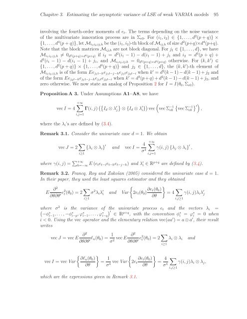
Chapitre 3. Estimating the asymptotic variance of LSE of weak VARMA models 95
involving the fourth-order moments of et. The terms depending on the noise variance
of the multivariate innovation process are in Σe0. For (i1,i2) ∈ {1,...,d 2 (p+q)} ×
{1,...,d 4 (p+q)}, letMi1i2,ij,h be the(i1,i2)-th block ofMij,h of sized 2 (p+q)×d 4 (p+q).
Note that the block matrices Mij,h are not block diagonal. For j1 ∈ {1,...,d}, we have
Mi1i2,ij,h = 0 d 2 (p+q)×d 4 (p+q) if i2 = d 2 (i1 − 1) − d(i1 − 1) + j1 and i2 = d 3 (p + q) +
d 2 (i1 − 1) − d(i1 − 1) + j1, and Mi1i2,ij,h = 0d 2 (p+q)×d 4 (p+q) otherwise. For (k,k ′ ) ∈
{1,...,d 2 (p+q)} × {1,...,d 4 (p+q)} and j2 ∈ {1,...,d}, the (k,k ′ )-th element of
Mi1i2,ij,h is of the form Eej1t−hej1t−j−hej1tej2t−i when k ′ = d 2 (k−1)−d(k−1)+j2 and
of the form Eej2t−hej1t−j−hej1tej2t−i when k ′ = d 3 (p+q)+d 2 (k−1)−d(k−1)+j2, and
zero otherwise. We now state an analog of Proposition 2 for I = I(θ0,Σe0).
PropositionA 3. Under Assumptions A1–A8, we have
vecI = 4
+∞
i,j=1
Γ(i,j) Id ⊗λ ′ j
where the λi’s are defined by (3.4).
⊗{Id ⊗λ ′ i}
vec vecΣ −1
e0
Remark 3.1. Consider the univariate case d = 1. We obtain
vecJ = 2
{λi ⊗λi} ′
i≥1
and vecI = 4
σ 4
+∞
i,j=1
−1 ′
vecΣe0 ,
γ(i,j){λj ⊗λi} ′ ,
where γ(i,j) = +∞
h=−∞ E(etet−iet−het−j−h) and λ ′ i ∈ Rp+q are defined by (3.4).
Remark 3.2. Francq, Roy and Zakoïan (2005) considered the univariate case d = 1.
In their paper, they used the least squares estimator and they obtained
E ∂2
∂θ∂θ ′e2t (θ0) = 2
σ 2 λiλ ′
i and Var 2et(θ0) ∂et(θ0)
= 4
∂θ
γ(i,j)λiλ ′ j
i≥1
where σ2 is the variance of the univariate process et and the vectors λi
=
∗ −φi−1 ,...,−φ ∗ i−p ,ϕ∗i−1 ,...,ϕ∗ ′ p+q ∗
i−q ∈ R , with the convention φi = ϕ∗ i = 0 when
i < 0. Using the vec operator and the elementary relation vec(aa ′ ) = a⊗a ′ , their result
writes
vecJ = vecE ∂2
∂θ∂θ ′ℓn(θ0) = 1
σ
∂ℓn(θ0)
vecI = vec Var
∂θ
2 vecE ∂2
i,j≥1
∂θ∂θ ′e2t (θ0) = 2
λi ⊗λi and
i≥1
= 1
∂et(θ0)
vec Var 2et =
σ4 ∂θ
4
σ4 which are the expressions given in Remark 3.1.
γ(i,j)λi ⊗λj,
i,j≥1