THÈSE Estimation, validation et identification des modèles ARMA ...

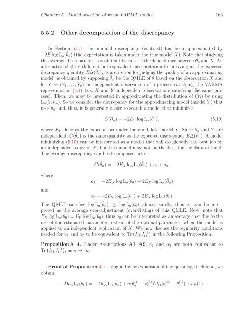
Chapitre 5. Model selection of weak VARMA models 163
5.5.2 Other decomposition of the discrepancy
In Section 5.5.1, the minimal discrepancy (contrast) has been approximated by
−2ElogLn( ˆ θn) (the expectation is taken under the true model X). Note that studying
this average discrepancy is too difficult because of the dependance between ˆ θn andX. An
alternative slightly different but equivalent interpretation for arriving at the expected
discrepancy quantity E∆( ˆ θn), as a criterion for judging the quality of an approximating
model, is obtained by supposing ˆ θn be the QMLE of θ based on the observation X and
let Y = (Y1,...,Yn) be independent observation of a process satisfying the VARMA
representation (5.1) (i.e. X and Y independent observations satisfying the same process).
Then, we may be interested in approximating the distribution of (Yt) by using
Ln(Y, ˆ θn). So we consider the discrepancy for the approximating model (model Y ) that
uses ˆ θn and, thus, it is generally easier to search a model that minimizes
C( ˆ θn) = −2EY logLn( ˆ θn), (5.10)
where EY denotes the expectation under the candidate model Y . Since ˆ θn and Y are
independent, C( ˆ θn) is the same quantity as the expected discrepancy E∆( ˆ θn). A model
minimizing (5.10) can be interpreted as a model that will do globally the best job on
an independent copy of X, but this model may not be the best for the data at hand.
The average discrepancy can be decomposed into
where
and
C( ˆ θn) = −2EX logLn( ˆ θn)+a1 +a2,
a1 = −2EX logLn(θ0)+2EX logLn( ˆ θn)
a2 = −2EY logLn( ˆ θn)+2EX logLn(θ0).
The QMLE satisfies logLn( ˆ θn) ≥ logLn(θ0) almost surely, thus a1 can be interpreted
as the average over-adjustment (over-fitting) of this QMLE. Now, note that
EX logLn(θ0) = EY logLn(θ0), thus a2 can be interpreted as an average cost due to the
use of the estimated parameter instead of the optimal parameter, when the model is
applied to an independent replication of X. We now discuss the regularity conditions
needed for a1 and a2 to be equivalent to Tr I11J −1
11 in the following Proposition.
PropositionA 4. Under Assumptions A1–A9, a1 and a2 are both equivalent to
Tr I11J −1
11 , as n → ∞.
Proof of Proposition 4 : Using a Taylor expansion of the quasi log-likelihood, we
obtain
−2logLn(θ0) = −2logLn( ˆ θn)+n( ˆ θ (1)
n −θ(1)
0 )′ J11( ˆ θ (1)
n −θ(1)
0 )+oP(1).