Equações Diferenciais Ordinárias (notas de aula) - Unesp
Equações Diferenciais Ordinárias (notas de aula) - Unesp
Equações Diferenciais Ordinárias (notas de aula) - Unesp

You also want an ePaper? Increase the reach of your titles
YUMPU automatically turns print PDFs into web optimized ePapers that Google loves.
4.2 Equação homogênea com coeficientes constantes(b) k 1 e k 2 são números reais e iguais (k 1 = k 2 )(c) k 1 e k 2 são números complexos.Analisemos cada caso por separado.4.2.1 Raízes distintasSe d > 0 então as raízes k 1 e k 2 são reais e distintas. Neste casok 1 = −p + √ d2e a solução geral <strong>de</strong> (4.13) é dada por4.2.2 Raízes iguaisek 1 = −p − √ d2x(t) = c 1 e k 1t + c 2 e k 2t , c 1 , c 2 ∈ R.Se d = 0, então k 1 = k 2 = − p 2 ∈ R e x 1(t) = e k 1t é solução <strong>de</strong> (4.13).Afirmação. x 2 (t) = te k 1t é solução <strong>de</strong> (4.13).De fato,ẋ 2 (t) = k 1 te k 1t + e k 1t = k 1 x 2 (t) + x 1 (t) (4.15)ẍ 2 (t) = k 1 ẋ 2 (t) + k 1 x 1 (t) (4.16)Da equação (4.15) temos x 1 (t) = ẋ 2 (t) − k 1 x 2 (t). Substituindo esta equaçãoem (4.16) obtemosGerman Lozada CruzMatemática-IBILCEIBILCE-SJRPo que implica queẍ 2 (t) = k 1 ẋ 2 (t) + k 1 (ẋ 2 (t) − k 1 x 2 (t)) = 2k 1 ẋ 2 (t) − k 2 1x 2 (t)= −pẋ 2 (t) − p24 x 2(t)= −pẋ 2 (t) − qx 2 (t)ẍ 2 (t) + pẋ 2 (t) + qx 2 (t) = 0.Isto prova a afirmação.99