Energy and Human Ambitions on a Finite Planet, 2021a

3 Population 34
which is really just a repeat of Eq. 3.1, where r takes the place of
ln(1 + p).
Example 3.2.2 Paralleling the deer population scenario from Example
3.2.1, ifwesetr 0.5, <strong>and</strong> have a population of P 100 adult deer
(half female), Eq. 3.3 says that Ṗ 50, meaning the population will
change by 50 units. 10
We could then use Eq. 3.4 to determine the population after 4 years:
P 100e 0.5·4 ≈ 739.
Let’s say that a given forest can support an ultimate number of deer,
labeled Q, in steady state, while the current population is labeled P.
The difference, Q − P is the “room” available for growth, which we
might think of as being tied to available resources. Once P Q, no more
resources are available to support growth.
Definition 3.2.2 The term “carrying capacity” is often used to describe
Q: the population supportable by the environment. The carrying capacity
(Q) for human population on Earth is not an agreed-upon number, <strong>and</strong> in
any case it is a strong function of lifestyle choices <strong>and</strong> resource dependence.
Q − P quantifies a growth-limiting mechanism by representing available
room. One way to incorporate this feature into our growth rate equation
is to make the rate of growth look like
Ṗ Q − P rP. (3.5)
Q
We have multiplied the original rate of rP by a term that changes the
effective growth rate r → r(Q − P)/Q. When P is small relative to Q,
the effective rate is essentially the original r. But the effective growth
rate approaches zero as P approaches Q. In other words, growth slows
down <strong>and</strong> hits zero when the population reaches its final saturation
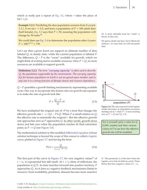
point, as P → Q (see Figure 3.6).
The mathematical solution to this modified differential equation (whose
solution technique is beyond the scope of this course) is called a logistic
curve, plotted in Figure 3.7 <strong>and</strong> having the form
10: A more adorable term for “units” is
fawns, in this case.
We ignore death rate here, but it effectively
reduces r in ways that we will encounter
later.
growth rate
0
r
population (P)
Figure 3.6: The rate of growth in the logistic
model decreases as population increases,
starting out at r when P 0 <strong>and</strong> reaching
zero as P → Q (see Eq. 3.5).
Q
Try it yourself: pick a value for Q
(1,000, maybe) <strong>and</strong> then various
values of P to see how the effective
growth rate will be modified.
P(t)
Q
1 + e −r(t−t 0) . (3.6)
The first part of the curve in Figure 3.7, for very negative values 11 of
t − t 0 , is exponential but still small. At t t 0 (time of inflection), the
population is Q/2. As time marches forward into positive territory, P
approaches Q. As it does so, negative feedback mechanisms (limits to
resource/food availability, predation, disease) become more assertive
11: The parameter t 0 is the time when the
logistic curve hits its halfway point. Times
before this have negative values of t − t 0 .
© 2021 T. W. Murphy, Jr.; Creative Commons Attribution-NonCommercial 4.0 International Lic.;
Freely available at: https://escholarship.org/uc/energy_ambitions.