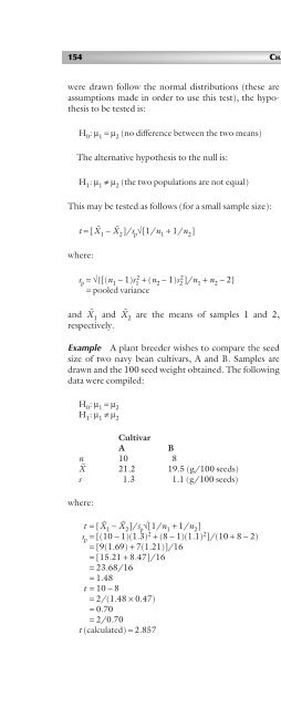
- Page 2:
Principles of Plant Genetics and Br
- Page 6:
Principles of Plant Genetics and Br
- Page 10:
Industry highlights boxes, vii Indu
- Page 14:
Industry highlights boxes Chapter 1
- Page 18:
Industry highlights box authors Acq
- Page 22:
Plant breeding is an art and a scie
- Page 26:
The author expresses sincere gratit
- Page 32:
Section 1 Historical perspectives a
- Page 36:
4 CHAPTER 1 accomplish astonishing
- Page 40:
6 CHAPTER 1 modifying the crop prod
- Page 44:
8 CHAPTER 1 Table 1.2 Selected mile
- Page 48:
10 CHAPTER 1 one season. Furthermor
- Page 52:
12 CHAPTER 1 Figure 1 Dr Norman Bor
- Page 56:
14 CHAPTER 1 agrochemicals. Recent
- Page 60:
Section 2 General biological concep
- Page 64:
18 CHAPTER 2 discovered. As will be
- Page 68:
20 CHAPTER 2 antiquity is establish
- Page 72:
22 CHAPTER 2 cultivation in areas a
- Page 76:
24 CHAPTER 2 Table 2.1 Characterist
- Page 80:
26 CHAPTER 2 Table 2.2 An operation
- Page 84:
28 CHAPTER 2 elite germplasm or adv
- Page 88:
30 CHAPTER 2 identify the most prom
- Page 92:
32 CHAPTER 2 Research Institute (SC
- Page 96:
34 CHAPTER 2 Part A Please answer t
- Page 100:
36 CHAPTER 3 out that when plants a
- Page 104:
38 CHAPTER 3 Table 3.2 Number of ch
- Page 108:
40 CHAPTER 3 AA × aa (a) A × a Aa
- Page 112:
42 CHAPTER 3 (a) PP × pp Pp 100% (
- Page 116:
44 CHAPTER 3 AB Ab aB ab (a) Parent
- Page 120:
46 CHAPTER 3 lifeblood of plant bre
- Page 124:
48 CHAPTER 3 -A=T- 5′ 3′ 5′ 5
- Page 128:
50 CHAPTER 3 Expression of genetic
- Page 132:
52 CHAPTER 3 Enhancer region subuni
- Page 136:
54 CHAPTER 3 Part A Please answer t
- Page 140:
56 CHAPTER 4 may be capable of self
- Page 144:
58 CHAPTER 4 Death Seed Reproductiv
- Page 148:
60 CHAPTER 4 Table 4.1 Pollination
- Page 152:
62 CHAPTER 4 homozygous and therefo
- Page 156:
64 CHAPTER 4 price of hybrid seed.
- Page 160:
66 CHAPTER 4 (a) (b) Figure 1 (a) A
- Page 164:
68 CHAPTER 4 only the desired polle
- Page 168:
70 CHAPTER 4 used to make a self-in
- Page 172:
72 CHAPTER 4 Male-fertile RfRf or R
- Page 176:
Section 3 Germplasm issues Chapter
- Page 180:
76 CHAPTER 5 Kingdom Division Class
- Page 184:
78 CHAPTER 5 may be classified into
- Page 188:
80 CHAPTER 5 plant breeding. As pre
- Page 192:
82 CHAPTER 5 both DNA strands; and
- Page 196:
84 CHAPTER 5 100% 50% (a) 100% 50%
- Page 200:
86 CHAPTER 5 Part B Please answer t
- Page 204:
88 CHAPTER 6 programs is the steady
- Page 208:
90 CHAPTER 6 What is genetic vulner
- Page 212:
92 CHAPTER 6 Table 1 Conservation m
- Page 216:
94 CHAPTER 6 Table 3 Varieties regi
- Page 220:
96 CHAPTER 6 linkage maps and a new
- Page 224:
98 CHAPTER 6 Approaches to germplas
- Page 228:
100 CHAPTER 6 resources. Curators o
- Page 232:
102 CHAPTER 6 difficult for users t
- Page 236:
104 CHAPTER 6 and Agricultural Orga
- Page 240:
106 CHAPTER 6 Table 6.2 Germplasm h
- Page 244:
Section 4 Genetic analysis in plant
- Page 248:
110 CHAPTER 7 underlying genetic co
- Page 252:
112 CHAPTER 7 of genes as 1 : n : n
- Page 256:
114 CHAPTER 7 may be toxic in addit
- Page 260:
116 CHAPTER 7 any male gamete of th
- Page 264:
118 CHAPTER 7 B C D E A B C E A I I
- Page 268:
120 CHAPTER 7 heterozygous plants g
- Page 272:
122 CHAPTER 8 2 Absence of linkage.
- Page 276:
124 CHAPTER 8 Table 8.2 As the numb
- Page 280:
126 CHAPTER 8 pollen from a random
- Page 284: 128 CHAPTER 8 environmental varianc
- Page 288: 130 CHAPTER 8 This estimate is fair
- Page 292: 132 CHAPTER 8 in a decline in both
- Page 296: 134 CHAPTER 8 Tandem selection In t
- Page 300: 136 CHAPTER 8 day. This process was
- Page 304: 138 CHAPTER 8 Frequency (%) 40 30 2
- Page 308: 140 CHAPTER 8 ability, the procedur
- Page 312: 142 CHAPTER 8 family are evaluated,
- Page 316: 144 CHAPTER 8 A × B A F2 B F2 A F2
- Page 320: Purpose and expected outcomes Stati
- Page 324: 148 CHAPTER 9 Concept of statistica
- Page 328: 150 CHAPTER 9 Using data in Table 9
- Page 332: 152 CHAPTER 9 Covariance =−2.45 C
- Page 338: Multivariate statistics in plant br
- Page 342: PC3 (15.8%) PC2 (30.72%) 0.10 0.05
- Page 346: Canonical function II 0.8 0.6 0.4 0
- Page 350: Discriminant function analysis Disc
- Page 354: Section 5 Tools in plant breeding C
- Page 358: Applications of crossing in plant b
- Page 362: emasculation is not a universal req
- Page 366: However, in other crosses, the F 2
- Page 370: Single cross A × B AB Proportion A
- Page 374: 3 Creation of new alloploids. Wide
- Page 378: SEXUAL HYBRIDIZATION AND WIDE CROSS
- Page 382: SEXUAL HYBRIDIZATION AND WIDE CROSS
- Page 386:
R. C. Buckner and his colleagues su
- Page 390:
Purpose and expected outcomes The c
- Page 394:
TISSUE CULTURE AND THE BREEDING OF
- Page 398:
previously described. Sometimes, to
- Page 402:
fraction of androgenic grains devel
- Page 406:
Introduction Sergey Chalyk TISSUE C
- Page 410:
TISSUE CULTURE AND THE BREEDING OF
- Page 414:
TISSUE CULTURE AND THE BREEDING OF
- Page 418:
only be maintained by vegetative pr
- Page 422:
Sexually reproductive Apomict New c
- Page 426:
Purpose and expected outcomes It wa
- Page 430:
the same plant. However, the dual c
- Page 434:
1 The ends of the segment may be di
- Page 438:
mutagen frequency is desired, the e
- Page 442:
Introduction F. Laurens MUTAGENESIS
- Page 446:
Climatic adaptation MUTAGENESIS IN
- Page 450:
MUTAGENESIS IN PLANT BREEDING 211 K
- Page 454:
Part A Please answer the following
- Page 458:
Triticum monococcum (2n = 2x = 14)
- Page 462:
(a) (b) A B A B a b a b A B A B a b
- Page 466:
Table 13.4 Genetics of autoploids.
- Page 470:
of sterility because of the odd chr
- Page 474:
(a) (b) (c) Figure 1 (a) Germinated
- Page 478:
Figure 2 In vitro regenerated plant
- Page 482:
(AABBDDRR, 2n = 8x = 56), but it re
- Page 486:
(in alloploids) or homologous (in a
- Page 490:
Purpose and expected outcomes Genes
- Page 494:
and expression (including codon usa
- Page 498:
1 Efficient plant regeneration syst
- Page 502:
Structural defect in the gene const
- Page 506:
sequence analysis. It is an applica
- Page 510:
Analysis BIOTECHNOLOGY IN PLANT BRE
- Page 514:
BIOTECHNOLOGY IN PLANT BREEDING 243
- Page 518:
of genes of known functions. Three
- Page 522:
source of the gene is a wild germpl
- Page 526:
ands for identification may minimiz
- Page 530:
location, genetic effects, and the
- Page 534:
3 Germplasm evaluation. Markers can
- Page 538:
Engineering pest resistance To date
- Page 542:
Purpose and expected outcomes Intel
- Page 546:
the key functions of a patent is to
- Page 550:
The development of truly new and un
- Page 554:
Ethics in plant breeding Manipulati
- Page 558:
Introduction ISSUES IN THE APPLICAT
- Page 562:
ISSUES IN THE APPLICATION OF BIOTEC
- Page 566:
Overview of the regulation of the U
- Page 570:
Table 15.2 Some viral-coated protei
- Page 574:
conditions. Further, these phenotyp
- Page 578:
there is no inherent health risk in
- Page 582:
esistance concerns (or “collatera
- Page 586:
Damage to economic interest (market
- Page 590:
Section 6 Classic methods of plant
- Page 594:
Open-pollinated cultivars Contrary
- Page 598:
Common plant breeding notations Pla
- Page 602:
(a) Year 1 Year 2 Year 3 (b) Source
- Page 606:
2 Cultivars developed for a discrim
- Page 610:
especially where readily identifiab
- Page 614:
Comments 1 Growing parents, making
- Page 618:
Comments Generation Year 1 P 1 × P
- Page 622:
3 Natural selection may increase fr
- Page 626:
5 Every plant originates from a dif
- Page 630:
1 year BREEDING SELF-POLLINATED SPE
- Page 634:
BREEDING SELF-POLLINATED SPECIES 30
- Page 638:
Year 1 Year 2 F 1 Year 3 Year 4 Yea
- Page 642:
2 Extensive advanced testing is not
- Page 646:
Applications One of the earliest ap
- Page 650:
species (maize) and has been a majo
- Page 654:
Purpose and expected outcomes As pr
- Page 658:
epistatic interactions enhance the
- Page 662:
Season 1 Source population C 0 Seas
- Page 666:
Procedure: cycle 1 This is the same
- Page 670:
Advantages and disadvantages The ma
- Page 674:
(a) (b) Figure 1 Examples of (a) Po
- Page 678:
Figure 3 Range of seed development
- Page 682:
Applications The scheme has been us
- Page 686:
stems from several biological facto
- Page 690:
Factors affecting the performance o
- Page 694:
7 Give a specific disadvantage of m
- Page 698:
Other notable advances in the breed
- Page 702:
BREEDING HYBRID CULTIVARS 337 ducin
- Page 706:
BREEDING HYBRID CULTIVARS 339 for c
- Page 710:
of interest. As Falconer indicated,
- Page 714:
patterns derived from the same open
- Page 718:
(a) (b) Seed parent (male-sterile)
- Page 722:
Table 18.1 Calculating heat units a
- Page 726:
such as sugarcane (most commercial
- Page 730:
Section 7 Selected breeding objecti
- Page 734:
water utilization, photoperiod, har
- Page 738:
expense of the rest of the plant. N
- Page 742:
usually results from one component
- Page 746:
Figure 3 Field trials demonstrating
- Page 750:
References Concept of yield plateau
- Page 754:
Shatter-sensitive cultivars are sus
- Page 758:
Nature, types, and economic importa
- Page 762:
Purpose and expected outcomes Plant
- Page 766:
elative to a benchmark. A genotype
- Page 770:
Types of genetic resistance The com
- Page 774:
General considerations for breeding
- Page 778:
for most middling resistance. It sh
- Page 782:
pathogen to give resistance), was c
- Page 786:
BREEDING FOR RESISTANCE TO DISEASES
- Page 790:
BREEDING FOR RESISTANCE TO DISEASES
- Page 794:
5 The plant or cell overproduces th
- Page 798:
Purpose and expected outcomes Clima
- Page 802:
ultimately its productivity and eco
- Page 806:
Breeding for drought resistance Dro
- Page 810:
drought. Consequently, phenotypic s
- Page 814:
BREEDING FOR RESISTANCE TO ABIOTIC
- Page 818:
More N partitioned to leaves before
- Page 822:
interruption in normal germination,
- Page 826:
Table 21.1 Relative salt tolerance
- Page 830:
toxicities of economic importance t
- Page 834:
Acevedo, E., and E. Fereres. 1993.
- Page 838:
Table 22.1 Essential amino acids th
- Page 842:
BREEDING COMPOSITIONAL TRAITS AND A
- Page 846:
Figure 1 Farmer (left) and research
- Page 850:
the presence of β-carotene, but no
- Page 854:
and cell walls are degraded. There
- Page 858:
milling, extraction of oil, starch
- Page 862:
Section 8 Cultivar release and comm
- Page 866:
in two stages. The first stage, cal
- Page 870:
genotype is reduced. This raises th
- Page 874:
Different models of ANOVA are used
- Page 878:
Table 23.2 Stability analysis. PERF
- Page 882:
PERFORMANCE EVALUATION FOR CROP CUL
- Page 886:
esources available (land, seed, lab
- Page 890:
Advantages 1 It is the simplest of
- Page 894:
Mapping populations have additional
- Page 898:
Purpose and expected outcomes The u
- Page 902:
Funk Columbiana Farm Seed Germain
- Page 906:
Joe W. Burton SEED CERTIFICATION AN
- Page 910:
Registered seed Registered seed is
- Page 914:
Canada’s Plant Breeders’ Rights
- Page 918:
Seed certification process There ar
- Page 922:
Table 24.1 Information on a seed ta
- Page 926:
Boswell, V.R. 1961. The importance
- Page 930:
property is a major one in plant br
- Page 934:
important issues to be considered i
- Page 938:
Soybean Soybean research is conduct
- Page 942:
INTERNATIONAL PLANT BREEDING EFFORT
- Page 946:
Selected accomplishments The impact
- Page 950:
national entities. More importantly
- Page 954:
Cicarelli contest that most farmers
- Page 958:
EMERGING CONCEPTS IN PLANT BREEDING
- Page 962:
EMERGING CONCEPTS IN PLANT BREEDING
- Page 966:
Principles of organic plant breedin
- Page 970:
Part II Breeding selected crops Cha
- Page 974:
Adaptation Wheat is best adapted to
- Page 978:
are less successful, being of poor
- Page 982:
Introduction BREEDING WHEAT 477 Ind
- Page 986:
Host plant resistance to disease an
- Page 990:
Greenhouse nursery Breeders may use
- Page 994:
when the production area is isolate
- Page 998:
Taxonomy Kingdom Plantae Subkingdom
- Page 1002:
encloses the soft starch at the cen
- Page 1006:
Designated ms 1 , ms 2 ,...ms n , o
- Page 1010:
F. J. Betrán Texas A&M University,
- Page 1014:
Development of hybrids BREEDING COR
- Page 1018:
chambers may be used for experiment
- Page 1022:
orer. A chemical found in corn with
- Page 1026:
A British sea captain brought rice
- Page 1030:
while awnless is conditioned by an
- Page 1034:
Figure 1 Rice panicle being prepare
- Page 1038:
Figure 5 A foundation seed field of
- Page 1042:
emoved with forceps, the cut may be
- Page 1046:
Taxonomy Kingdom Plantae Subkingdom
- Page 1050:
green midrib because of the presenc
- Page 1054:
BREEDING SORGHUM 513 Kansas State U
- Page 1058:
Summer Year 5 Summer Year 7 Summer
- Page 1062:
covered with the bag. Pollination s
- Page 1066:
Taxonomy Kingdom Plantae Subkingdom
- Page 1070:
and brown being dominant over gray.
- Page 1074:
BREEDING SOYBEAN 523 easily selecte
- Page 1078:
BREEDING SOYBEAN 525 An advantage o
- Page 1082:
Common breeding objectives 1 Grain
- Page 1086:
Taxonomy Kingdom Plantae Subkingdom
- Page 1090:
Program objectives Charles Simpson
- Page 1094:
BREEDING PEANUT 533 lines in hopes
- Page 1098:
for emasculation, which is done in
- Page 1102:
Taxonomy Kingdom Plantae Subkingdom
- Page 1106:
Evolution of the modern potato crop
- Page 1110:
BREEDING POTATO 541 Table 1 The Sco
- Page 1114:
(berries) called potato balls. The
- Page 1118:
6 Potato tuber quality improvement.
- Page 1122:
grown in America, Africa, Asia, and
- Page 1126:
Introduction Don L. Keim BREEDING C
- Page 1130:
BREEDING COTTON 551 are grown in tr
- Page 1134:
economically important traits has b
- Page 1138:
Part B Please answer the following
- Page 1142:
Central dogma: The underlying model
- Page 1146:
Mitosis: The process of nuclear div
- Page 1150:
Chapter 1 http://www.foodfirst.org/
- Page 1154:
Imperial unit Metric conversion Vol
- Page 1158:
complex inheritance, 42 composite c
- Page 1162:
minor gene resistance, 371 minor ge
- Page 1166:
technology protection system (TPS),


