Principles of Plant Genetics and Breeding

424 CHAPTER 23
example, a significant G × year interaction cannot be
exploited because the climatic conditions that generate
year-to-year environmental variation are not
known in advance. Consequently, the analysis of
multiple environment yield trials should focus primarily
on G × location interactions, the other interaction
being considered in terms of yield stability.
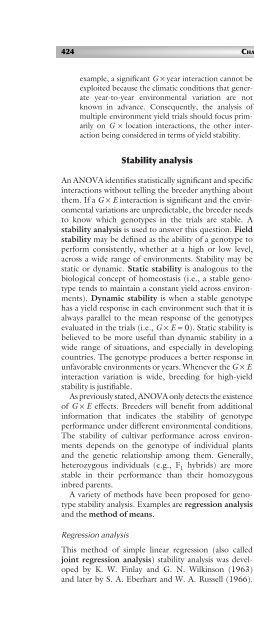
Stability analysis
An ANOVA identifies statistically significant and specific
interactions without telling the breeder anything about
them. If a G × E interaction is significant and the environmental
variations are unpredictable, the breeder needs
to know which genotypes in the trials are stable. A
stability analysis is used to answer this question. Field
stability may be defined as the ability of a genotype to
perform consistently, whether at a high or low level,
across a wide range of environments. Stability may be
static or dynamic. Static stability is analogous to the
biological concept of homeostasis (i.e., a stable genotype
tends to maintain a constant yield across environments).
Dynamic stability is when a stable genotype
has a yield response in each environment such that it is
always parallel to the mean response of the genotypes
evaluated in the trials (i.e., G × E = 0). Static stability is
believed to be more useful than dynamic stability in a
wide range of situations, and especially in developing
countries. The genotype produces a better response in
unfavorable environments or years. Whenever the G × E
interaction variation is wide, breeding for high-yield
stability is justifiable.
As previously stated, ANOVA only detects the existence
of G × E effects. Breeders will benefit from additional
information that indicates the stability of genotype
performance under different environmental conditions.
The stability of cultivar performance across environments
depends on the genotype of individual plants
and the genetic relationship among them. Generally,
heterozygous individuals (e.g., F 1 hybrids) are more
stable in their performance than their homozygous
inbred parents.
A variety of methods have been proposed for genotype
stability analysis. Examples are regression analysis
and the method of means.
Regression analysis
This method of simple linear regression (also called
joint regression analysis) stability analysis was developed
by K. W. Finlay and G. N. Wilkinson (1963)
and later by S. A. Eberhart and W. A. Russell (1966).
It is preceded by an ANOVA to assess the significance
of G × E. The breeder proceeds to the next step of
regression analysis only if the G × E interaction is
significant.
Statistically, the observed performance (Y ij ) of the
ith genotype (i = 1,..., 5) in the jth environment
(j = 1,..., e), may be expressed as:
Y ij =µ+g i + e j + ge ij +ε ij
where µ =grand mean over all genotypes and environments,
g i = additive contribution of the ith genotype
(calculated as the deviation from µ of the mean of the ith
genotype averaged over all environments), e j = additive
environmental contribution of the jth environment
(calculated as the deviation µ of the mean of the jth
environment averaged over all genotypes), ge ij = G × E
interaction of the ith genotype in the jth environment,
and ε ij = error term attached to the ith genotype
in the jth environment. The regression coefficient for a
specific genotype is obtained by regressing its observed
Y ij value against the corresponding mean of the jth
environment.
If the yield was conducted over a wide range of environments,
and hence a wide range of yields obtained, it
is reasonable to assume that the individual trial means
sufficiently summarize the effects of the environments.
The mean performance of each genotype over all the
test environments constitutes the environmental index
(Table 23.2). In effect, this method of analysis produces
a scale of environmental quality. The results for each
genotype are plotted, trial by trial, against trial means, to
obtain a regression line. According to Eberhart and
Russell, an average performing genotype will have a
regression coefficient of 1.0 and deviations from regression
of 0.0, since it will tend to agree with the means.
However the genotypes that were responsible for the
G × E interactions detected in the ANOVA, will have
slopes that are unequal to unity. Furthermore, a genotype
that is unresponsive to environments (i.e., a stable
performer) will have a low slope (b < 1), while a genotype
that is responsive to environments (i.e., an unstable
performer) will have a steep slope (b > 1).
The regression analysis technique has certain limitations,
both physiological and statistical, that can result
in inaccurate interpretation and recommendations for
cultivar release. For example, the use of mean yield in
each environment as an environmental index flouts
the statistical requirement of an independent variable.
Also, when regression lines do not adequately represent
data, the point of intersection of these lines
has little biological meaning, unless considered with