Application and Optimisation of the Spatial Phase Shifting ...

More documents

Recommendations

Info

8 Statistical Properties of Speckle Patterns together. Another interesting possibility of measuring speckle phases is the Fizeau configuration reported in [Mol90a,b]. HeNe laser BS MO2 L2 M2/SP NDF P2 MO1 L1 M1 CCD P1 BSC Fig. 2.1: Optical set-up for generation of large speckles and phase measurement by SPS. Abbreviations: BS(C), beam splitter (cube), NDF, neutral density filter, MO, microscope objectives, L, lenses, M, mirrors, SP, scattering plate. The laser beam is divided, expanded by microscope objectives of the same type and made convergent again by lenses of the same type (f=120 mm); we call the path with component index 1 the reference path. To adjust the speckle size, the scattering plate (matt white painted metal) is fit and L2 is slid back or forth to produce the proper spot diameter (in our case, 3.1 mm). The neutral density filter is chosen so as to maximise the modulation of the speckle interferogram. Here, we set R/I7:6. Then SP is replaced by M2 and L1 is moved so that P1 and P2 acquire the same distance from the CCD chip; thus the curvatures of the two spherical waves are matched. By rotating M1, the spatial phase shift can be adjusted with no de-focusing: P1 is merely shifted sideways as M1 is rotated. The lateral offset between P1 and P2 determines the fringe density on the CCD, i.e., the spatial phase shift. An explanation of the underlying geometry can be found in Chapter 3.4.1. Uniting the two fields involves sending at least one of them through glass, which introduces spherical aberrations. Here, we subject both waves to almost the same alteration by using a beam splitter cube with high-planarity surfaces. The attainable flatness of the measured wavefront depends on the quality of the optical components; a residual error of about λ/4 was found, which is tolerable for our range of speckle sizes. Also, any misalignment of the spatial phase shift will generate an additional phase ramp; but since it is linear, we can easily detect and remove it by the fitting procedure described in Chapter 4.2. Once this calibration is done, M2 must be replaced by SP again, and their surfaces should be in exactly the same position. For this purpose, we used an auxiliary adjustment frame that was removed afterwards. The scattered light is weakly de-polarised (1:10); but as we will see, very little impact on the statistics is found (for a detailed survey on partially polarised speckle fields, see [Bar85]). The laser beam has a
2.1 Experimental set-up 9 Gaussian intensity profile; after expanding, only its innermost part is being transmitted by the lenses, so that we can approximate the illuminated scattering spot by a circle of uniform brightness. Moving the CCD camera away from BSC offers the additional possibility to scan the speckle field in the direction of propagation, which we label z. It is then not necessary to re-align the spatial phase shift: the ratio of fringe density to speckle size, being the relative resolution of the speckle phase maps, will remain constant. For a series of images with varying fringe density, the phase maps can most conveniently be obtained by the Fourier transform method (see Chapter 6.5). A non-integer number of carrier fringes will leave a residual global phase ramp after the FT evaluation. This bogus wavefront tilt must be removed if we are to measure speckle phases only; and again, the "fringe" fitting algorithm of Chapter 4.2 is capable of finding the global ramp that we have to subtract. The CCD camera used for this experiment was a SONY XC-75 with interline transfer sensor (dust cover removed) and a resolution of 736576 pixels of (8.5 µm) 2 each; we call d p = 8.5 µm the pixel size. the video signal was digitised to 8 bits (256 grey levels) by a Data Translation DT3852B-2 frame grabber, driven by the camera's pixel clock. 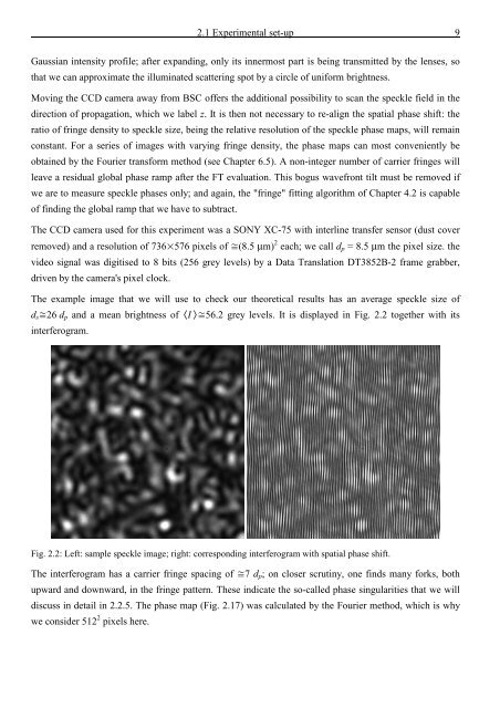The example image that we will use to check our theoretical results has an average speckle size of d s 26 d p and a mean brightness of I 56.2 grey levels. It is displayed in Fig. 2.2 together with its interferogram. Fig. 2.2: Left: sample speckle image; right: corresponding interferogram with spatial phase shift. The interferogram has a carrier fringe spacing of 7 d p ; on closer scrutiny, one finds many forks, both upward and downward, in the fringe pattern. These indicate the so-called phase singularities that we will discuss in detail in 2.2.5. The phase map (Fig. 2.17) was calculated by the Fourier method, which is why we consider 512 2 pixels here.
Page 1 and 2: Application and Optimisation of the
Page 3 and 4: Table of Contents 1 1 INTRODUCTION
Page 5 and 6: 3 1 Introduction The present era of
Page 7 and 8: Introduction 5 retrieval can help t
Page 9: 7 2 Statistical Properties of Speck
Page 13 and 14: 2.2 First-order speckle statistics
Page 35 and 36: 2.3 Second-order speckle statistics
Page 49 and 50: 47 3 Electronic or Digital Speckle
Page 51 and 52: 3.1 Subtraction-mode ESPI 49 some 4
Page 53 and 54: 3.2 Phase-shifting ESPI 51 filled u
Page 55 and 56: 3.2 Phase-shifting ESPI 53 known si
Page 57 and 58: 3.2 Phase-shifting ESPI 55 α n =α
Page 59 and 60: 3.2 Phase-shifting ESPI 57 But reme
Page 61 and 62:
3.2 Phase-shifting ESPI 59 ϕ ϕ O,
Page 63 and 64:
3.2 Phase-shifting ESPI 61 These fo
Page 65 and 66:
3.2 Phase-shifting ESPI 63 ∞ ~ ~
Page 67 and 68:
3.2 Phase-shifting ESPI 65 ∞ N
Page 69 and 70:
3.2 Phase-shifting ESPI 67 The spec
Page 71 and 72:
3.2 Phase-shifting ESPI 69 − 0. 2
Page 73 and 74:
3.2 Phase-shifting ESPI 71 ν x 0 i
Page 75 and 76:
3.2 Phase-shifting ESPI 73 to think
Page 77 and 78:
3.3 Temporal phase shifting 75 Agai
Page 79 and 80:
3.3 Temporal phase shifting 77 addi
Page 81 and 82:
3.4 Spatial phase shifting 79 which
Page 83 and 84:
3.4 Spatial phase shifting 81 3.4.1
Page 85 and 86:
3.4 Spatial phase shifting 83 cross
Page 87 and 88:
3.4 Spatial phase shifting 85 Fig.
Page 89 and 90:
3.4 Spatial phase shifting 87 arran
Page 91 and 92:
3.4 Spatial phase shifting 89 infor
Page 93 and 94:
3.4 Spatial phase shifting 91 frequ
Page 95 and 96:
3.4 Spatial phase shifting 93 altho
Page 97 and 98:
3.4 Spatial phase shifting 95 error
Page 99:
3.4 Spatial phase shifting 97 Since
Page 102 and 103:
100 Quantification of displacement-
Page 104 and 105:
Page 106 and 107:
Page 108 and 109:
Page 110 and 111:
Page 112 and 113:
110
Page 114 and 115:
112 Comparison of noise in phase ma
Page 116 and 117:
Page 118 and 119:
Page 120 and 121:
Page 122 and 123:
Page 124 and 125:
Page 126 and 127:
Page 128 and 129:
Page 130 and 131:
Page 132 and 133:
Page 134 and 135:
Page 136 and 137:
134 Improvements on SPS intensity o
Page 138 and 139:
136 Improvements on SPS 0.14 σ d /
Page 140 and 141:
138 Improvements on SPS we are conc
Page 142 and 143:
140 Improvements on SPS 6.2 Modifie
Page 144 and 145:
Page 146 and 147:
144 Improvements on SPS Fig. 6.7 te
Page 148 and 149:
146 Improvements on SPS Finally, bo
Page 150 and 151:
148 Improvements on SPS To use the
Page 152 and 153:
150 Improvements on SPS The improve
Page 154 and 155:
152 Improvements on SPS On the whol
Page 156 and 157:
154 Improvements on SPS In classica
Page 158 and 159:
156 Improvements on SPS generally n
Page 160 and 161:
Page 162 and 163:
160 Improvements on SPS uncertain,
Page 164 and 165:
162 Improvements on SPS To obtain p
Page 166 and 167:
164 Improvements on SPS Fig. 6.22:
Page 168 and 169:
166 Improvements on SPS This proced
Page 170 and 171:
168 Improvements on SPS 6.7.2 Long-
Page 172 and 173:
170 Improvements on SPS Fig. 6.28:
Page 174 and 175:
172 Improvements on SPS the heater
Page 176 and 177:
174
Page 178 and 179:
176 Summary method to search for a
Page 180 and 181:
178
Page 182 and 183:
180 References [Bot97] [Bra87] [Bro
Page 184 and 185:
182 References [Ett97] [Fac93] [Far
Page 186 and 187:
184 References [Har94] [Her96] [Het
Page 188 and 189:
186 References [Kuj89] [Kuj91a] [Ku
Page 190 and 191:
188 References [McLa86] [Mer83] J.
Page 192 and 193:
190 References [Rav99] I. Raveh, E.
Page 194 and 195:
192 References [Sur98b] [Sur98c] [S
Page 196 and 197:
194
Page 198 and 199:
196 Appendix A: Counting events and
Page 200 and 201:
198 Appendix B: Real-time phase cal
Page 202 and 203:
200 Appendix C: Derivation of inten
Page 204 and 205:
I 1 a r g ( S ~ ( ) ) 202 Appendix
Page 206 and 207:
204 Appendix D: Alternative error-c
Page 208 and 209:
206
Page 210 and 211:
208
Page 212 and 213:
210 The author List of publications
Page 214:
212
show all

Application and Optimisation of the Spatial Phase Shifting ...

You also want an ePaper? Increase the reach of your titles

Delete template?

Save as template?