Application and Optimisation of the Spatial Phase Shifting ...

3.4 Spatial phase shifting 91
frequencies. The difference is solely that those regions of the frequency plane where there is no signal,
and hence relatively little spectral power, are quite a bit more noisy.
ν N
1.57
0.785
ν y
0
0
ν
0 1 2 3 x /ν 0x 4
-0.785
–ν N
2 3 4|0 1 2 ν x /ν 0x -1.57
Fig. 3.33: Left: bsc(ν x ,ν y ) for (3.18) as calculated from (3.73), with 0 black and 2π white; note that ν x =ν y = 0 is
in the centre of the image. Right: bsc(ν x ) for (3.18) (black) and (3.19) (white); average of 50 rows from
the small black frame on the left.
To the right, the plot of bsc(ν x ) as output by (3.18) (black) and (3.19) (white) does indeed show that both
compare quite well with the corresponding graph in Fig. 3.13. The high noise around ν x = 0 and ν x = 2ν N
reflects the suppression of I b , i.e. the fact that ~ ~ S ( 0 ) = C(
0)
= 0.
It is interesting to note that, in agreement
with the larger absolute filter output of (3.18), the susceptibility to noise is indeed somewhat lower than
for (3.19); but this affects a frequency range that produces large errors anyway, so that the difference in
performance will be very small. For this case of α=90°, we therefore conclude that the utilisation of
different sets of pixels for different representations of the 3-sample 90° formula does not invalidate the
theoretical considerations in 3.2.2.3.
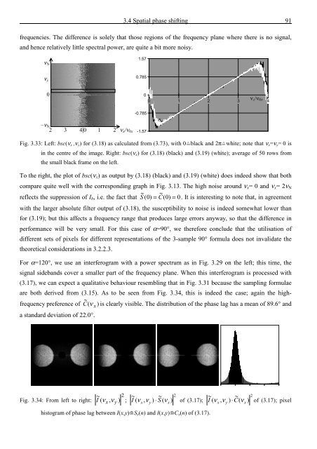
For α=120°, we use an interferogram with a power spectrum as in Fig. 3.29 on the left; this time, the
signal sidebands cover a smaller part of the frequency plane. When this interferogram is processed with
(3.17), we can expect a qualitative behaviour resembling that in Fig. 3.31 because the sampling formulae
are both derived from (3.15). As to be seen from Fig. 3.34, this is indeed the case; again the highfrequency
preference of C
~ ( ν ) is clearly visible. The distribution of the phase lag has a mean of 89.6° and
a standard deviation of 22.0°.
x
Fig. 3.34: From left to right: ~ 2 ~ ~
2
~ ~ 2
( ν , ν ) ; I ( ν , ν ) ⋅ S ( ν ) of (3.17); I ( ν , ν ) ⋅ C(
ν ) of (3.17); pixel
I x y
x y x
histogram of phase lag between I(x,y)¡S x (n) and I(x,y)¡C x (n) of (3.17).
x y x